The writeexcel rubygem can be used to create a cross-platform Excel binary file. Multiple worksheets can be added to a workbook and formatting can be applied to cells. Text, numbers, formulas, hyperlinks, images and charts can be written to the cells.
Writeexcel Rubygem and this reference is ported from Spreadsheet::WriteExcel-2.3.7 module of perl. If you have any problem or question, please contact me.
writeexcel - Write to a cross-platform Excel binary file.
This document refers to version 0.6.6 of writeexcel, released February 2, 2010.
To write a string, a formatted string, a number and a formula to the first worksheet in an Excel workbook called ruby.xls:
    # -*- coding:utf-8 -*-
    require 'writeexcel'

    # Create a new Excel workbook
    workbook = WriteExcel.new('ruby.xls')

    # Add a worksheet
    worksheet = workbook.add_worksheet

    #  Add and define a format
    format = workbook.add_format  # Add a format
    format.set_bold
    format.set_color('red')
    format.set_align('center')

    # Write a formatted and unformatted string, row and column notation.
    col = row = 0
    worksheet.write(row, col, 'Hi Excel!', format)
    worksheet.write(1,   col, 'Hi Excel!')

    # Write a number and a formula using A1 notation
    worksheet.write('A3', 1.2345)
    worksheet.write('A4', '=SIN(PI()/4)')

    workbook.close
The writeexcel rubygem can be used to create a cross-platform Excel binary file. Multiple worksheets can be added to a workbook and formatting can be applied to cells. Text, numbers, formulas, hyperlinks, images and charts can be written to the cells.
The file produced by this module is compatible with Excel 97, 2000, 2002, 2003 and 2007.
The module will work on the majority of Windows, UNIX and Mac platforms. Generated files are also compatible with the Linux/UNIX spreadsheet applications Gnumeric and OpenOffice.org.
This module cannot be used to write to an existing Excel file.
This library is converted from Spreadsheet::WriteExcel-2.3.7 module of Perl.
writeexcel tries to provide an interface to as many of Excel's features as possible. As a result there is a lot of documentation to accompany the interface and it can be difficult at first glance to see what it important and what is not. So for those of you who prefer to assemble Ikea furniture first and then read the instructions, here are three easy steps:
1. Create a new Excel workbook (i.e. file) using new.
2. Add a worksheet to the new workbook using add_worksheet.
3. Write to the worksheet using write.
4. Close workbook using close.
Like this:
    # -*- coding:utf-8 -*-
    require 'writeexcel'                  # Step 0

    workbook = WriteExcel.new('ruby.xls') # Step 1
    worksheet   = workbook.add_worksheet  # Step 2
    worksheet.write('A1', 'Hi Excel!')    # Step 3
    workbook.close                        # Step 4
You must create source file in UTF-8, and run ruby in UTF-8 mode by using -Ku option(1.8) or magic comment(1.9).
This will create an Excel file called ruby.xls with a single worksheet and the text 'Hi Excel!' in the relevant cell. And that's it. Okay, so there is actually a zeroth step as well, but require goes without saying. There are also many examples that come with the distribution and which you can use to get you started.
Those of you who read the instructions first and assemble the furniture afterwards will know how to proceed. ;-)
The WriteExcel module provides an object oriented interface to a new Excel workbook. The following methods are available through a new workbook.
    new
    add_worksheet
    add_format
    add_chart
    add_chart_ext
    close
    compatibility_mode
    set_properties
    define_name
    set_tempdir
    set_custom_color
    sheets
    set_1904
    set_codepage
A new Excel workbook is created using the new constructor which accepts either a filename or a io object as a parameter. The following example creates a new Excel file based on a filename:
    workbook  = WriteExcel.new('filename.xls')
    worksheet = workbook.add_worksheet
    worksheet.write(0, 0, 'Hi Excel!')
    workbook.close
Here are some other examples of using new:
    workbook1 = WriteExcel.new(filename)
    workbook2 = WriteExcel.new('/tmp/filename.xls')
    workbook3 = WriteExcel.new("c:\\tmp\\filename.xls")
    workbook4 = WriteExcel.new('c:\tmp\filename.xls')
The last two examples demonstrates how to create a file on DOS or Windows where it is necessary to either escape the directory separator \ or to use single quotes to ensure that it isn't interpolated.
The new constructor returns a WriteExcel object that you can use to add worksheets and store data.
If the file cannot be created, due to file permissions or some other reason, new raises Exception of Errno::EXXX.
You can also pass a IO object to the new constructor.:
    require 'stringio'

    io = StringIO.new
    workbook = WriteExcel.new(io)  # After workbook.close, you can get excel data as io.string
And, you can also pass default format properties.
workbook = WriteExcel.new(filename, :font => 'Courier New', :size => 11)
See the "CELL FORMATTING" section for more details about Format properties and how to set them.
At least one worksheet should be added to a new workbook. A worksheet is used to write data into cells:
    worksheet1 = workbook.add_worksheet             # Sheet1
    worksheet2 = workbook.add_worksheet('Foglio2')  # Foglio2
    worksheet3 = workbook.add_worksheet('Data')     # Data
    worksheet4 = workbook.add_worksheet             # Sheet4
If sheetname is not specified the default Excel convention will be followed, i.e. Sheet1, Sheet2, etc. The name_utf16be parameter is optional, see below.
The worksheet name must be a valid Excel worksheet name, i.e. it cannot contain any of the following characters,
[ ] : * ? / \
and it must be less than 32 characters. In addition, you cannot use the same, case insensitive, sheetname for more than one worksheet.
You can specify UTF-16BE worksheet names using an additional optional parameter:
    name = [0x263a].pack('n')
    worksheet = workbook.add_worksheet(name, true)   # Smiley
The add_format method can be used to create new Format objects which are used to apply formatting to a cell. You can either define the properties at creation time via a hash of property values or later via method calls.
    format1 = workbook.add_format(:font => 'Courier New')  # Set properties at creation
    format2 = workbook.add_format                          # Set properties later
See the "CELL FORMATTING" section for more details about Format properties and how to set them.
This method is use to create a new chart either as a standalone worksheet (the default) or as an embeddable object that can be inserted into a worksheet via the insert_chart Worksheet method.
chart = workbook.add_chart( :type => 'column' )
The properties that can be set are:
    :type     (required)
    :name     (optional)
    :name_utf16be (optional)
    :embedded (optional)
:type
This is a required parameter. It defines the type of chart that will be created.
chart = workbook.add_chart( :type => 'Chart::line' )
The available types are:
    'Chart::area'
    'Chart::bar'
    'Chart::column'
    'Chart::line'
    'Chart::pie'
    'Chart::scatter'
    'Chart::stock'
:name
Set the name for the chart sheet. The name property is optional and if it isn't supplied will default to Chart1 .. n. The name must be a valid Excel worksheet name. See add_worksheet for more details on valid sheet names. The :name property can be omitted for embedded charts.
chart = workbook.add_chart( :type => 'Chart::line', :name => 'Results Chart' )
:name_utf16be
if :name is UTF-16BE format, pass true as :name_utf16be
:embedded
Specifies true that the Chart object will be inserted in a worksheet via the insert_chart Worksheet method. It is an error to try insert a Chart that doesn't have this flag set.
    chart = workbook.add_chart( :type => 'Chart::line', :embedded => true )

    # Configure the chart.
    ...

    # Insert the chart into the a worksheet.
    worksheet.insert_chart( 'E2', chart )
See WriteExcel::Chart for details on how to configure the chart object once it is created. See also the chart_*.rb programs in the examples directory of the distro.
This method is use to include externally generated charts in a WriteExcel file.
chart = workbook.add_chart_ext('chart01.bin', 'Chart1')
This feature is semi-deprecated in favour of the "native" charts created using add_chart. Read external_charts.txt in the external_charts directory of the distro for a full explanation.
The close method is used to explicitly close an Excel file.
workbook.close
An explicit close is required if the file must be closed prior to performing some external action on it such as copying it, reading its size or attaching it to an email.
In general, if you create a file with a size of 0 bytes or you fail to create a file you need to call close.
This method is used to improve compatibility with third party applications that read Excel files.
workbook.compatibility_mode
An Excel file is comprised of binary records that describe properties of a spreadsheet. Excel is reasonably liberal about this and, outside of a core subset, it doesn't require every possible record to be present when it reads a file. This is also true of Gnumeric and OpenOffice.Org Calc.
WriteExcel takes advantage of this fact to omit some records in order to minimise the amount of data stored in memory and to simplify and speed up the writing of files. However, some third party applications that read Excel files often expect certain records to be present. In "compatibility mode" WriteExcel writes these records and tries to be as close to an Excel generated file as possible.
Applications that require compatibility_mode are Apache POI, Apple Numbers, and Quickoffice on Nokia, Palm and other devices. You should also use compatibility_mode if your Excel file will be used as an external data source by another Excel file.
If you encounter other situations that require compatibility_mode, please let me know.
It should be noted that compatibility_mode requires additional data to be stored in memory and additional processing. This incurs a memory and speed penalty and may not be suitable for very large files (>20MB).
You must call compatibility_mode before calling add_worksheet.
The set_properties method can be used to set the document properties of the Excel file created by WriteExcel. These properties are visible when you use the File.Properties menu option in Excel and are also available to external applications that read or index windows files.
The properties should be passed as a hash of values as follows:
    workbook.set_properties(
        :title    => 'This is an example spreadsheet',
        :comments => 'Created with Ruby and writeexcel',
    )
The properties that can be set are:
    :title
    :subject
    :author
    :manager
    :company
    :category
    :keywords
    :comments
User defined properties are not supported due to effort required.
Usually WriteExcel allows you to use UTF-16. However, document properties don't support UTF-16 for these type of strings.
In order to promote the usefulness of Ruby and the writeexcel rubygems consider adding a comment such as the following when using document properties:
    workbook.set_properties(
        ...,
        :comments => 'Created with Ruby and writeexcel',
        ...,
    )
See also the properties.rb and properties_jp.rbprogram in the examples directory of the distro.
This method is used to defined a name that can be used to represent a value, a single cell or a range of cells in a workbook.
    workbook.define_name('Exchange_rate', '=0.96')
    workbook.define_name('Sales',         '=Sheet1!G1:H10')
    workbook.define_name('Sheet2!Sales',  '=Sheet2!G1:G10')
See the defined_name.rb program in the examples dir of the distro.
Note: This currently a beta feature. More documentation and examples will be added.
For speed and efficiency WriteExcel stores worksheet data in temporary files prior to assembling the final workbook.
If WriteExcel is unable to create these temporary files it will store the required data in memory. This can be slow for large files.
The problem occurs mainly with IIS on Windows although it could feasibly occur on Unix systems as well. The problem generally occurs because the default temp file directory is defined as C:/ or some other directory that IIS doesn't provide write access to.
To check if this might be a problem on a particular system you can run a simple test program with -w or use warnings. This will generate a warning if the module cannot create the required temporary files:
    #!/usr/bin/ruby -w

    require 'writeexcel'

    workbook  = WriteExcel.new('test.xls')
    worksheet = workbook.add_worksheet
To avoid this problem the set_tempdir method can be used to specify a directory that is accessible for the creation of temporary files.
Even if the default temporary file directory is accessible you may wish to specify an alternative location for security or maintenance reasons:
    workbook.set_tempdir('/tmp/writeexcel')
    workbook.set_tempdir('c:\windows\temp\writeexcel')
The directory for the temporary file must exist, set_tempdir will not create a new directory.
One disadvantage of using the set_tempdir method is that on some Windows systems it will limit you to approximately 800 concurrent tempfiles. This means that a single program running on one of these systems will be limited to creating a total of 800 workbook and worksheet objects. You can run multiple, non-concurrent programs to work around this if necessary.
The set_custom_color method can be used to override one of the built-in palette values with a more suitable colour.
The value for index should be in the range 8..63, see "COLOURS IN EXCEL".
The default named colours use the following indices:
     8   =>   black
     9   =>   white
    10   =>   red
    11   =>   lime
    12   =>   blue
    13   =>   yellow
    14   =>   magenta
    15   =>   cyan
    16   =>   brown
    17   =>   green
    18   =>   navy
    20   =>   purple
    22   =>   silver
    23   =>   gray
    33   =>   pink
    53   =>   orange
A new colour is set using its RGB (red green blue) components. The red, green and blue values must be in the range 0..255. You can determine the required values in Excel using the Tools.Options.Colors.Modify dialog.
The set_custom_color workbook method can also be used with a HTML style #rrggbb hex value:
    workbook.set_custom_color(40, 255,  102,  0   ) # Orange
    workbook.set_custom_color(40, 0xFF, 0x66, 0x00) # Same thing
    workbook.set_custom_color(40, '#FF6600'       ) # Same thing

    font = workbook.add_format(:color => 40) # Use the modified colour
The return value from set_custom_color is the index of the colour that was changed:
    ferrari = workbook.set_custom_color(40, 216, 12, 12)

    format  = workbook.add_format(
                                        :bg_color => ferrari,
                                        :pattern  => 1,
                                        :border   => 1
                                 )
The sheets method returns a list, or a sliced list, of the worksheets in a workbook.
If no arguments are passed the method returns a list of all the worksheets in the workbook. This is useful if you want to repeat an operation on each worksheet:
    workbook.sheets.each do |worksheet|
      print worksheet.name
    end
You can also specify a slice list to return one or more worksheet objects:
    worksheet = workbook.sheets(0)
    worksheet.write('A1', 'Hello')
Or since return value from sheets is a reference to a worksheet object you can write the above example as:
workbook.sheets(0).write('A1', 'Hello')
The following example returns the first and last worksheet in a workbook:
    workbook.sheets(0, -1).each do |worksheet|
       # Do something
    end
Excel stores dates as real numbers where the integer part stores the number of days since the epoch and the fractional part stores the percentage of the day. The epoch can be either 1900 or 1904. Excel for Windows uses 1900 and Excel for Macintosh uses 1904. However, Excel on either platform will convert automatically between one system and the other.
WriteExcel stores dates in the 1900 format by default. If you wish to change this you can call the set_1904 workbook method. You can query the current value by calling the get_1904 workbook method. This returns false for 1900 and true for 1904.
See also "DATES AND TIME IN EXCEL" for more information about working with Excel's date system.
In general you probably won't need to use set_1904.
The default code page or character set used by WriteExcel is ANSI. This is also the default used by Excel for Windows. Occasionally however it may be necessary to change the code page via the set_codepage method.
Changing the code page may be required if your are using WriteExcel on the Macintosh and you are using characters outside the ASCII 128 character set:
    workbook.set_codepage(1) # ANSI, MS Windows
    workbook.set_codepage(2) # Apple Macintosh
The set_codepage method is rarely required.
A new worksheet is created by calling the add_worksheet method from a workbook object:
    worksheet1 = workbook.add_worksheet
    worksheet2 = workbook.add_worksheet
The following methods are available through a new worksheet:
    write
    write_number
    write_string
    write_utf16be_string
    write_utf16le_string
    write_blank
    write_row
    write_col
    write_date_time
    write_url
    write_url_range
    write_formula
    store_formula
    repeat_formula
    write_comment
    show_comments
    add_write_handler
    insert_image
    insert_chart
    data_validation
    get_name
    activate
    select
    hide
    set_first_sheet
    protect
    set_selection
    set_row
    set_column
    outline_settings
    freeze_panes
    split_panes
    merge_range
    set_zoom
    right_to_left
    hide_zero
    set_tab_color
    autofilter
WriteExcel supports two forms of notation to designate the position of cells: Row-column notation and A1 notation.
Row-column notation uses a zero based index for both row and column while A1 notation uses the standard Excel alphanumeric sequence of column letter and 1-based row. For example:
    (0, 0)      # The top left cell in row-column notation.
    ('A1')      # The top left cell in A1 notation.

    (1999, 29)  # Row-column notation.
    ('AD2000')  # The same cell in A1 notation.
Row-column notation is useful if you are referring to cells programmatically:
    (0 .. 9).each { |i|
       worksheet.write(i, 0, 'Hello') # Cells A1 to A10
    }
A1 notation is useful for setting up a worksheet manually and for working with formulas:
    worksheet.write('H1', 200)
    worksheet.write('H2', '=H1+1')
In formulas and applicable methods you can also use the A:A column notation:
worksheet.write('A1', '=SUM(B:B)')
For simplicity, the parameter lists for the worksheet method calls in the following sections are given in terms of row-column notation. In all cases it is also possible to use A1 notation.
Note: in Excel it is also possible to use a R1C1 notation. This is not supported by WriteExcel.
Excel makes a distinction between data types such as strings, numbers, blanks, formulas and hyperlinks. To simplify the process of writing data the write method acts as a general alias for several more specific methods:
    write_string
    write_number
    write_blank
    write_formula
    write_url
    write_row
    write_col
The general rule is that if the data looks like a something then a something is written. Here are some examples in both row-column and A1 notation:
    # Same as:
    worksheet.write(0, 0, 'Hello'                ) # write_string
    worksheet.write(1, 0, 'One'                  ) # write_string
    worksheet.write(2, 0,  2                     ) # write_number
    worksheet.write(3, 0,  3.00001               ) # write_number
    worksheet.write(4, 0,  ""                    ) # write_blank
    worksheet.write(5, 0,  ''                    ) # write_blank
    worksheet.write(6, 0,  nil                   ) # write_blank
    worksheet.write(7, 0                         ) # write_blank
    worksheet.write(8, 0,  'http://www.ruby.com/') # write_url
    worksheet.write('A9',  'ftp://ftp.ruby.org/' ) # write_url
    worksheet.write('A10', 'internal:Sheet1!A1'  ) # write_url
    worksheet.write('A11', 'external:c:\foo.xls' ) # write_url
    worksheet.write('A12', '=A3 + 3*A4'          ) # write_formula
    worksheet.write('A13', '=SIN(PI()/4)'        ) # write_formula
    worksheet.write('A14', array                 ) # write_row
    worksheet.write('A15', [array]               ) # write_col
The "looks like" rule is defined by regular expressions:
write_number if token is a number based on the following regex: token =~ /^([+-]?)(?=\d|\.\d)\d*(\.\d*)?([Ee]([+-]?\d+))?/.
write_blank if token is nil or a blank string: nil, "" or ''.
write_url if token is a http, https, ftp or mailto URL based on the following regexes: token =~ m|^[fh]tt?ps?://| or token =~ m|^mailto:|.
write_url if token is an internal or external sheet reference based on the following regex: token =~ m[^(in|ex)ternal:].
write_formula if the first character of token is "=".
write_row if token is an array.
write_col if token is an array of array.
write_string if none of the previous conditions apply.
The format parameter is optional. It should be a valid Format object, see "CELL FORMATTING":
    format = workbook.add_format
    format.set_bold
    format.set_color('red')
    format.set_align('center')

    worksheet.write(4, 0, 'Hello', format) # Formatted string
The write method will ignore empty strings or nil tokens unless a format is also supplied. As such you needn't worry about special handling for empty or nil values in your data. See also the write_blank method.
The write methods return:
    0 for success.
   -1 for insufficient number of arguments.
   -2 for row or column out of bounds.
   -3 for string too long.
Write an integer or a float to the cell specified by row and column:
    worksheet.write_number(0, 0,  123456)
    worksheet.write_number('A2',  2.3451)
See the note about "Cell notation". The format parameter is optional.
In general it is sufficient to use the write method.
Write a string to the cell specified by row and column:
    worksheet.write_string(0, 0, 'Your text here' )
    worksheet.write_string('A2', 'or here' )
The maximum string size is 32767 characters. However the maximum string segment that Excel can display in a cell is 1000. All 32767 characters can be displayed in the formula bar.
The format parameter is optional.
In general it is sufficient to use the write method. However, you may sometimes wish to use the write_string method to write data that looks like a number but that you don't want treated as a number. For example, zip codes or phone numbers:
    # Write as a plain string
    worksheet.write_string('A1', '01209')
However, if the user edits this string Excel may convert it back to a number. To get around this you can use the Excel text format @:
    # Format as a string. Doesn't change to a number when edited
    format1 = workbook.add_format(:num_format => '@')
    worksheet.write_string('A2', '01209', format1)
See also the note about "Cell notation".
This method is used to write UTF-16BE strings to a cell in Excel.
UTF-16 data can be changed from little-endian to big-endian format (and vice-versa) as follows:
utf16be = [utf16le.unpack('v*')].pack('n*')
Write a blank cell specified by row and column:
worksheet.write_blank(0, 0, format)
This method is used to add formatting to a cell which doesn't contain a string or number value.
Excel differentiates between an "Empty" cell and a "Blank" cell. An "Empty" cell is a cell which doesn't contain data whilst a "Blank" cell is a cell which doesn't contain data but does contain formatting. Excel stores "Blank" cells but ignores "Empty" cells.
As such, if you write an empty cell without formatting it is ignored:
    worksheet.write('A1',  nil, format) # write_blank
    worksheet.write('A2',  nil        ) # Ignored
This seemingly uninteresting fact means that you can write arrays of data without special treatment for nil or empty string values.
See the note about "Cell notation".
The write_row method can be used to write a 1D or 2D array of data in one go. This is useful for converting the results of a database query into an Excel worksheet. The write method is then called for each element of the data. For example:
    array      = ['awk', 'gawk', 'mawk']

    worksheet.write_row(0, 0, array)

    # The above example is equivalent to:
    worksheet.write(0, 0, array[0])
    worksheet.write(0, 1, array[1])
    worksheet.write(0, 2, array[2])
Note: For convenience the write method behaves in the same way as write_row if it is passed an array. Therefore the following two method calls are equivalent:
    worksheet.write_row('A1', array) # Write a row of data
    worksheet.write(    'A1', array) # Same thing
As with all of the write methods the format parameter is optional. If a format is specified it is applied to all the elements of the data array.
Array references within the data will be treated as columns. This allows you to write 2D arrays of data in one go. For example:
    eec =  [
                ['maggie', 'milly', 'molly', 'may'  ],
                [13,       14,      15,      16     ],
                ['shell',  'star',  'crab',  'stone']
           ]

    worksheet.write_row('A1', eec)
Would produce a worksheet as follows:
     -----------------------------------------------------------
    |   |    A    |    B    |    C    |    D    |    E    | ...
     -----------------------------------------------------------
    | 1 | maggie  | 13      | shell   | ...     |  ...    | ...
    | 2 | milly   | 14      | star    | ...     |  ...    | ...
    | 3 | molly   | 15      | crab    | ...     |  ...    | ...
    | 4 | may     | 16      | stone   | ...     |  ...    | ...
    | 5 | ...     | ...     | ...     | ...     |  ...    | ...
    | 6 | ...     | ...     | ...     | ...     |  ...    | ...
To write the data in a row-column order refer to the write_col method below.
Any nil values in the data will be ignored unless a format is applied to the data, in which case a formatted blank cell will be written. In either case the appropriate row or column value will still be incremented.
The write_row method returns the first error encountered when writing the elements of the data or zero if no errors were encountered. See the return values described for the write method above.
See also the write_arrays.rb program in the examples directory of the distro.
The write_col method can be used to write a 1D or 2D array of data in one go. This is useful for converting the results of a database query into an Excel worksheet. You must pass a reference to the array of data rather than the array itself. The write method is then called for each element of the data. For example:
    array      = ['awk', 'gawk', 'mawk']

    worksheet.write_col(0, 0, array)

    # The above example is equivalent to:
    worksheet.write(0, 0, array[0])
    worksheet.write(1, 0, array[1])
    worksheet.write(2, 0, array[2])
As with all of the write methods the format parameter is optional. If a format is specified it is applied to all the elements of the data array.
Array within the data will be treated as rows. This allows you to write 2D arrays of data in one go. For example:
    eec =  [
                ['maggie', 'milly', 'molly', 'may'  ],
                [13,       14,      15,      16     ],
                ['shell',  'star',  'crab',  'stone']
           ]

    worksheet.write_col('A1', \@eec)
Would produce a worksheet as follows:
     -----------------------------------------------------------
    |   |    A    |    B    |    C    |    D    |    E    | ...
     -----------------------------------------------------------
    | 1 | maggie  | milly   | molly   | may     |  ...    | ...
    | 2 | 13      | 14      | 15      | 16      |  ...    | ...
    | 3 | shell   | star    | crab    | stone   |  ...    | ...
    | 4 | ...     | ...     | ...     | ...     |  ...    | ...
    | 5 | ...     | ...     | ...     | ...     |  ...    | ...
    | 6 | ...     | ...     | ...     | ...     |  ...    | ...
To write the data in a column-row order refer to the write_row method above.
Any nil values in the data will be ignored unless a format is applied to the data, in which case a formatted blank cell will be written. In either case the appropriate row or column value will still be incremented.
As noted above the write method can be used as a synonym for write_row and write_row handles nested array as columns. Therefore, the following two method calls are equivalent although the more explicit call to write_col would be preferable for maintainability:
    worksheet.write_col('A1', array    ) # Write a column of data
    worksheet.write(    'A1', [ array ]) # Same thing
The write_col method returns the first error encountered when writing the elements of the data or zero if no errors were encountered. See the return values described for the write method above.
See also the write_arrays.rb program in the examples directory of the distro.
The write_date_time method can be used to write a date or time to the cell specified by row and column:
worksheet.write_date_time('A1', '2004-05-13T23:20', date_format)
The date_string should be in the following format:
yyyy-mm-ddThh:mm:ss.sss
This conforms to an ISO8601 date but it should be noted that the full range of ISO8601 formats are not supported.
The following variations on the date_string parameter are permitted:
    yyyy-mm-ddThh:mm:ss.sss         # Standard format
    yyyy-mm-ddT                     # No time
              Thh:mm:ss.sss         # No date
    yyyy-mm-ddThh:mm:ss.sssZ        # Additional Z (but not time zones)
    yyyy-mm-ddThh:mm:ss             # No fractional seconds
    yyyy-mm-ddThh:mm                # No seconds
Note that the T is required in all cases.
A date should always have a format, otherwise it will appear as a number, see "DATES AND TIME IN EXCEL" and "CELL FORMATTING". Here is a typical example:
    date_format = workbook.add_format(:num_format => 'mm/dd/yy')
    worksheet.write_date_time('A1', '2004-05-13T23:20', date_format)
Valid dates should be in the range 1900-01-01 to 9999-12-31, for the 1900 epoch and 1904-01-01 to 9999-12-31, for the 1904 epoch. As with Excel, dates outside these ranges will be written as a string.
See also the date_time.rb program in the examples directory of the distro.
Write a hyperlink to a URL in the cell specified by row and column. The hyperlink is comprised of two elements: the visible label and the invisible link. The visible label is the same as the link unless an alternative label is specified. The parameters label and the format are optional and their position is interchangeable.
The label is written using the write method. Therefore it is possible to write strings, numbers or formulas as labels.
There are four web style URI's supported: http://, https://, ftp:// and mailto::
    worksheet.write_url(0, 0,  'ftp://www.ruby.org/'                 )
    worksheet.write_url(1, 0,  'http://www.ruby.com/', 'Ruby home'   )
    worksheet.write_url('A3',  'http://www.ruby.com/', format        )
    worksheet.write_url('A4',  'http://www.ruby.com/', 'Ruby', format)
    worksheet.write_url('A5',  'mailto:cxn03651@ruby.org'            )
There are two local URIs supported: internal: and external:. These are used for hyperlinks to internal worksheet references or external workbook and worksheet references:
    worksheet.write_url('A6',  'internal:Sheet2!A1'                   )
    worksheet.write_url('A7',  'internal:Sheet2!A1',   format         )
    worksheet.write_url('A8',  'internal:Sheet2!A1:B2'                )
    worksheet.write_url('A9',  q{internal:'Sales Data'!A1}            )
    worksheet.write_url('A10', 'external:c:\temp\foo.xls'             )
    worksheet.write_url('A11', 'external:c:\temp\foo.xls#Sheet2!A1'   )
    worksheet.write_url('A12', 'external:..\..\..\foo.xls'            )
    worksheet.write_url('A13', 'external:..\..\..\foo.xls#Sheet2!A1'  )
    worksheet.write_url('A13', 'external:\\\\NETWORK\share\foo.xls'   )
All of the these URI types are recognised by the write method, see above.
Worksheet references are typically of the form Sheet1!A1. You can also refer to a worksheet range using the standard Excel notation: Sheet1!A1:B2.
In external links the workbook and worksheet name must be separated by the # character: external:Workbook.xls#Sheet1!A1'.
You can also link to a named range in the target worksheet. For example say you have a named range called my_name in the workbook c:\temp\foo.xls you could link to it as follows:
worksheet.write_url('A14', 'external:c:\temp\foo.xls#my_name')
Note, you cannot currently create named ranges with WriteExcel.
Excel requires that worksheet names containing spaces or non alphanumeric characters are single quoted as follows 'Sales Data'!A1.
Links to network files are also supported. MS/Novell Network files normally begin with two back slashes as follows \\NETWORK\etc. In order to generate this in a single or double quoted string you will have to escape the backslashes, '\\\\NETWORK\etc'.
If you are using double quote strings then you should be careful to escape anything that looks like a metacharacter. For more information see perlfaq5: Why can't I use "C:\temp\foo" in DOS paths?.
Finally, you can avoid most of these quoting problems by using forward slashes. These are translated internally to backslashes:
    worksheet.write_url('A14', "external:c:/temp/foo.xls"             )
    worksheet.write_url('A15', 'external://NETWORK/share/foo.xls'     )
See also, the note about "Cell notation".
This method is essentially the same as the write_url method described above. The main difference is that you can specify a link for a range of cells:
    worksheet.write_url(0, 0, 0, 3, 'ftp://www.ruby.org/'              )
    worksheet.write_url(1, 0, 0, 3, 'http://www.ruby.com/', 'Ruby home')
    worksheet.write_url('A3:D3',    'internal:Sheet2!A1'               )
    worksheet.write_url('A4:D4',    'external:c:\temp\foo.xls'         )
This method is generally only required when used in conjunction with merged cells. See the merge_range method and the merge property of a Format object, "CELL FORMATTING".
There is no way to force this behaviour through the write method.
The parameters string and the format are optional and their position is interchangeable. However, they are applied only to the first cell in the range.
See also, the note about "Cell notation".
Write a formula or function to the cell specified by row and column:
    worksheet.write_formula(0, 0, '=B3 + B4'  )
    worksheet.write_formula(1, 0, '=SIN(PI()/4)')
    worksheet.write_formula(2, 0, '=SUM(B1:B5)' )
    worksheet.write_formula('A4', '=IF(A3>1,"Yes", "No")'   )
    worksheet.write_formula('A5', '=AVERAGE(1, 2, 3, 4)'    )
    worksheet.write_formula('A6', '=DATEVALUE("1-Jan-2001")')
See the note about "Cell notation". For more information about writing Excel formulas see "FORMULAS AND FUNCTIONS IN EXCEL"
See also the section "Improving performance when working with formulas" and the store_formula and repeat_formula methods.
If required, it is also possible to specify the calculated value of the formula. This is occasionally necessary when working with non-Excel applications that don't calculated the value of the formula. The calculated value is added at the end of the argument list:
worksheet.write('A1', '=2+2', format, 4)
However, this probably isn't something that will ever need to do. If you do use this feature then do so with care.
The store_formula method is used in conjunction with repeat_formula to speed up the generation of repeated formulas. See "Improving performance when working with formulas" in "FORMULAS AND FUNCTIONS IN EXCEL".
The store_formula method pre-parses a textual representation of a formula and stores it for use at a later stage by the repeat_formula method.
store_formula carries the same speed penalty as write_formula. However, in practice it will be used less frequently.
The return value of this method is a scalar that can be thought of as a reference to a formula.
    sin = worksheet.store_formula('=SIN(A1)')
    cos = worksheet.store_formula('=COS(A1)')

    worksheet.repeat_formula('B1', sin, format, 'A1', 'A2')
    worksheet.repeat_formula('C1', cos, format, 'A1', 'A2')
Although store_formula is a worksheet method the return value can be used in any worksheet:
    now = worksheet.store_formula('=NOW')

    worksheet1.repeat_formula('B1', now)
    worksheet2.repeat_formula('B1', now)
    worksheet3.repeat_formula('B1', now)
The repeat_formula method is used in conjunction with store_formula to speed up the generation of repeated formulas. See "Improving performance when working with formulas" in "FORMULAS AND FUNCTIONS IN EXCEL".
In many respects repeat_formula behaves like write_formula except that it is significantly faster.
The repeat_formula method creates a new formula based on the pre-parsed tokens returned by store_formula. The new formula is generated by substituting pattern, replace pairs in the stored formula:
    formula = worksheet.store_formula('=A1 * 3 + 50')

    (0..99).each do |row|
      worksheet.repeat_formula(row, 1, formula, format, 'A1', 'A'.(row +1))
    end
It should be noted that repeat_formula doesn't modify the tokens. In the above example the substitution is always made against the original token, A1, which doesn't change.
As usual, you can use nil if you don't wish to specify a format:
    worksheet.repeat_formula('B2', formula, format, 'A1', 'A2')
    worksheet.repeat_formula('B3', formula, nil,    'A1', 'A3')
The substitutions are made from left to right and you can use as many pattern, replace pairs as you need. However, each substitution is made only once:
    formula = worksheet.store_formula('=A1 + A1')

    # Gives '=B1 + A1'
    worksheet.repeat_formula('B1', formula, nil, 'A1', 'B1')

    # Gives '=B1 + B1'
    worksheet.repeat_formula('B2', formula, nil, 'A1', 'B1', 'A1', 'B1')
Since the pattern is interpolated each time that it is used it is worth using the %q operator to quote the pattern.
worksheet.repeat_formula('B1', formula, format, %q/A1/, 'A2')
Care should be taken with the values that are substituted. The formula returned by repeat_formula contains several other tokens in addition to those in the formula and these might also match the pattern that you are trying to replace. In particular you should avoid substituting a single 0, 1, 2 or 3.
You should also be careful to avoid false matches. For example the following snippet is meant to change the stored formula in steps from =A1 + SIN(A1) to =A10 + SIN(A10).
    formula = worksheet.store_formula('=A1 + SIN(A1)')

    (1 .. 10).each do |row|
      worksheet.repeat_formula(row -1, 1, formula, nil,
                               'A1', "A#{row}",   #! Bad.
                               'A1', "A#{row}"    #! Bad.
                              )
    }
However it contains a bug. In the last iteration of the loop when row is 10 the following substitutions will occur:
    sub('A1', 'A10')    changes    =A1 + SIN(A1)     to    =A10 + SIN(A1)
    sub('A1', 'A10')    changes    =A10 + SIN(A1)    to    =A100 + SIN(A1) # !!
The solution in this case is to use a more explicit match such as /(?!A1\d+)A1/:
        worksheet.repeat_formula(row -1, 1, formula, nil,
                                    'A1', "A#{row}",
                                    /(?!A1\d+)A1/, "A#{row}"
                                  )
See also the repeat.rb program in the examples directory of the distro.
The write_comment method is used to add a comment to a cell. A cell comment is indicated in Excel by a small red triangle in the upper right-hand corner of the cell. Moving the cursor over the red triangle will reveal the comment.
The following example shows how to add a comment to a cell:
    worksheet.write        (2, 2, 'Hello')
    worksheet.write_comment(2, 2, 'This is a comment.')
As usual you can replace the row and column parameters with an A1 cell reference. See the note about "Cell notation".
    worksheet.write        ('C3', 'Hello')
    worksheet.write_comment('C3', 'This is a comment.')
In addition to the basic 3 argument form of write_comment you can pass in several optional key/value pairs to control the format of the comment. For example:
worksheet.write_comment('C3', 'Hello', :visible => 1, :author => 'Ruby')
Most of these options are quite specific and in general the default comment behaviour will be all that you need. However, should you need greater control over the format of the cell comment the following options are available:
    :encoding
    :author
    :author_encoding
    :visible
    :x_scale
    :width
    :y_scale
    :height
    :color
    :start_cell
    :start_row
    :start_col
    :x_offset
    :y_offset
This option is used to indicate that the comment string is encoded as UTF-16BE.
    comment = [0x263a].pack('n')   # UTF-16BE Smiley symbol

    worksheet.write_comment('C3', comment, :encoding => 1)
This option is used to indicate who the author of the comment is. Excel displays the author of the comment in the status bar at the bottom of the worksheet. This is usually of interest in corporate environments where several people might review and provide comments to a workbook.
worksheet.write_comment('C3', 'Atonement', :author => 'Ian McEwan')
This option is used to indicate that the author string is encoded as UTF-16BE.
This option is used to make a cell comment visible when the worksheet is opened. The default behaviour in Excel is that comments are initially hidden. However, it is also possible in Excel to make individual or all comments visible. In WriteExcel individual comments can be made visible as follows:
worksheet.write_comment('C3', 'Hello', :visible => 1)
It is possible to make all comments in a worksheet visible using the show_comments worksheet method (see below). Alternatively, if all of the cell comments have been made visible you can hide individual comments:
worksheet.write_comment('C3', 'Hello', :visible => 0)
This option is used to set the width of the cell comment box as a factor of the default width.
    worksheet.write_comment('C3', 'Hello', :x_scale => 2)
    worksheet.write_comment('C4', 'Hello', :x_scale => 4.2)
This option is used to set the width of the cell comment box explicitly in pixels.
worksheet.write_comment('C3', 'Hello', :width => 200)
This option is used to set the height of the cell comment box as a factor of the default height.
    worksheet.write_comment('C3', 'Hello', :y_scale => 2)
    worksheet.write_comment('C4', 'Hello', :y_scale => 4.2)
This option is used to set the height of the cell comment box explicitly in pixels.
worksheet.write_comment('C3', 'Hello', :height => 200)
This option is used to set the background colour of cell comment box. You can use one of the named colours recognised by WriteExcel or a colour index. See "COLOURS IN EXCEL".
    worksheet.write_comment('C3', 'Hello', :color => 'green')
    worksheet.write_comment('C4', 'Hello', :color => 0x35)    # Orange
This option is used to set the cell in which the comment will appear. By default Excel displays comments one cell to the right and one cell above the cell to which the comment relates. However, you can change this behaviour if you wish. In the following example the comment which would appear by default in cell D2 is moved to E2.
worksheet.write_comment('C3', 'Hello', :start_cell => 'E2')
This option is used to set the row in which the comment will appear. See the :start_cell option above. The row is zero indexed.
worksheet.write_comment('C3', 'Hello', :start_row => 0)
This option is used to set the column in which the comment will appear. See the :start_cell option above. The column is zero indexed.
worksheet.write_comment('C3', 'Hello', :start_col => 4)
This option is used to change the x offset, in pixels, of a comment within a cell:
worksheet.write_comment('C3', comment, :x_offset => 30)
This option is used to change the y offset, in pixels, of a comment within a cell:
worksheet.write_comment('C3', comment, :x_offset => 30)
You can apply as many of these options as you require.
Note about row height and comments. If you specify the height of a row that contains a comment then WriteExcel will adjust the height of the comment to maintain the default or user specified dimensions. However, the height of a row can also be adjusted automatically by Excel if the text wrap property is set or large fonts are used in the cell. This means that the height of the row is unknown to WriteExcel at run time and thus the comment box is stretched with the row. Use the set_row method to specify the row height explicitly and avoid this problem.
This method is used to make all cell comments visible when a worksheet is opened.
Individual comments can be made visible using the :visible parameter of the write_comment method (see above):
worksheet.write_comment('C3', 'Hello', :visible => 1)
If all of the cell comments have been made visible you can hide individual comments as follows:
worksheet.write_comment('C3', 'Hello', :visible => 0)
This method can be used to insert a image into a worksheet. The image can be in PNG, JPEG or BMP format. The x, y, scale_x and scale_y parameters are optional.
    worksheet1.insert_image('A1', 'ruby.bmp')
    worksheet2.insert_image('A1', '../images/ruby.bmp')
    worksheet3.insert_image('A1', 'c:\images\ruby.bmp')
The parameters x and y can be used to specify an offset from the top left hand corner of the cell specified by row and col. The offset values are in pixels.
worksheet1.insert_image('A1', 'ruby.bmp', 32, 10)
The default width of a cell is 63 pixels. The default height of a cell is 17 pixels. The pixels offsets can be calculated using the following relationships:
    Wp = int(12We)   if We <  1
    Wp = int(7We +5) if We >= 1
    Hp = int(4/3He)

    where:
    We is the cell width in Excels units
    Wp is width in pixels
    He is the cell height in Excels units
    Hp is height in pixels
The offsets can be greater than the width or height of the underlying cell. This can be occasionally useful if you wish to align two or more images relative to the same cell.
The parameters scale_x and scale_y can be used to scale the inserted image horizontally and vertically:
    # Scale the inserted image: width x 2.0, height x 0.8
    worksheet.insert_image('A1', 'ruby.bmp', 0, 0, 2, 0.8)
See also the images.rb program in the examples directory of the distro.
Note: you must call set_row or set_column before insert_image if you wish to change the default dimensions of any of the rows or columns that the image occupies. The height of a row can also change if you use a font that is larger than the default. This in turn will affect the scaling of your image. To avoid this you should explicitly set the height of the row using set_row if it contains a font size that will change the row height.
BMP images must be 24 bit, true colour, bitmaps. In general it is best to avoid BMP images since they aren't compressed.
This method can be used to insert a Chart object into a worksheet. The Chart must be created by the add_chart Workbook method and it must have the embedded option set.
    chart = workbook.add_chart( :type => 'Chart::Line', :embedded => true )

    # Configure the chart.
    ...

    # Insert the chart into the a worksheet.
    worksheet.insert_chart('E2', chart)
See add_chart for details on how to create the Chart object and WriteExcel::Chart for details on how to configure it. See also the chart_*.rb programs in the examples directory of the distro.
The x, y, scale_x and scale_y parameters are optional.
The parameters x and y can be used to specify an offset from the top left hand corner of the cell specified by row and col. The offset values are in pixels. See the insert_image method above for more information on sizes.
worksheet1.insert_chart('E2', chart, 3, 3)
The parameters scale_x and scale_y can be used to scale the inserted image horizontally and vertically:
    # Scale the width by 120% and the height by 150%
    worksheet.insert_chart('E2', chart, 0, 0, 1.2, 1.5)
The easiest way to calculate the required scaling is to create a test chart worksheet with WriteExcel. Then open the file, select the chart and drag the corner to get the required size. While holding down the mouse the scale of the resized chart is shown to the left of the formula bar.
Note: you must call set_row or set_column before insert_chart if you wish to change the default dimensions of any of the rows or columns that the chart occupies. The height of a row can also change if you use a font that is larger than the default. This in turn will affect the scaling of your chart. To avoid this you should explicitly set the height of the row using set_row if it contains a font size that will change the row height.
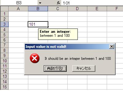
The data_validation method is used to construct an Excel data validation or to limit the user input to a dropdown list of values.
    worksheet.data_validation('B3',
        {
            :validate => 'integer',
            :criteria => '>',
            :value    => 100,
        })

    worksheet.data_validation('B5:B9',
        {
            :validate => 'list',
            :value    => ['open', 'high', 'close'],
        })
This method contains a lot of parameters and is described in detail in a separate section "DATA VALIDATION IN EXCEL".
See also the data_validate.rb program in the examples directory of the distro
The name method is used to retrieve the name of a worksheet. For example:
    workbook.sheets.each { |sheet|
      print sheet.name
    }
For reasons related to the design of WriteExcel and to the internals of Excel there is no name=(val) method. The only way to set the worksheet name is via the add_worksheet method.
The activate method is used to specify which worksheet is initially visible in a multi-sheet workbook:
    worksheet1 = workbook.add_worksheet('To')
    worksheet2 = workbook.add_worksheet('the')
    worksheet3 = workbook.add_worksheet('wind')

    worksheet3.activate
This is similar to the Excel VBA activate method. More than one worksheet can be selected via the select method, see below, however only one worksheet can be active.
The default active worksheet is the first worksheet.
The select method is used to indicate that a worksheet is selected in a multi-sheet workbook:
    worksheet1.activate
    worksheet2.select
    worksheet3.select
A selected worksheet has its tab highlighted. Selecting worksheets is a way of grouping them together so that, for example, several worksheets could be printed in one go. A worksheet that has been activated via the activate method will also appear as selected.
The hide method is used to hide a worksheet:
worksheet2.hide
You may wish to hide a worksheet in order to avoid confusing a user with intermediate data or calculations.
A hidden worksheet can not be activated or selected so this method is mutually exclusive with the activate and select methods. In addition, since the first worksheet will default to being the active worksheet, you cannot hide the first worksheet without activating another sheet:
    worksheet2.activate
    worksheet1.hide
The activate method determines which worksheet is initially selected. However, if there are a large number of worksheets the selected worksheet may not appear on the screen. To avoid this you can select which is the leftmost visible worksheet using set_first_sheet:
    (1..20).times { workbook.add_worksheet }

    worksheet21 = workbook.add_worksheet
    worksheet22 = workbook.add_worksheet

    worksheet21.set_first_sheet
    worksheet22.activate
This method is not required very often. The default value is the first worksheet.
The protect method is used to protect a worksheet from modification:
worksheet.protect
It can be turned off in Excel via the Tools.Protection.Unprotect Sheet menu command.
The protect method also has the effect of enabling a cell's locked and hidden properties if they have been set. A "locked" cell cannot be edited. A "hidden" cell will display the results of a formula but not the formula itself. In Excel a cell's locked property is on by default.
    # Set some format properties
    unlocked  = workbook.add_format(:locked => 0)
    hidden    = workbook.add_format(:hidden => 1)

    # Enable worksheet protection
    worksheet.protect

    # This cell cannot be edited, it is locked by default
    worksheet.write('A1', '=1+2')

    # This cell can be edited
    worksheet.write('A2', '=1+2', unlocked)

    # The formula in this cell isn't visible
    worksheet.write('A3', '=1+2', hidden)
See also the set_locked and set_hidden format methods in "CELL FORMATTING".
You can optionally add a password to the worksheet protection:
worksheet.protect('drowssap')
Note, the worksheet level password in Excel provides very weak protection. It does not encrypt your data in any way and it is very easy to deactivate. Therefore, do not use the above method if you wish to protect sensitive data or calculations. However, before you get worried, Excel's own workbook level password protection does provide strong encryption in Excel 97+. For technical reasons this will never be supported by WriteExcel.
This method can be used to specify which cell or cells are selected in a worksheet. The most common requirement is to select a single cell, in which case last_row and last_col can be omitted. The active cell within a selected range is determined by the order in which first and last are specified. It is also possible to specify a cell or a range using A1 notation. See the note about "Cell notation".
Examples:
    worksheet1.set_selection(3, 3)       # 1. Cell D4.
    worksheet2.set_selection(3, 3, 6, 6) # 2. Cells D4 to G7.
    worksheet3.set_selection(6, 6, 3, 3) # 3. Cells G7 to D4.
    worksheet4.set_selection('D4')       # Same as 1.
    worksheet5.set_selection('D4:G7')    # Same as 2.
    worksheet6.set_selection('G7:D4')    # Same as 3.
The default cell selections is (0, 0), 'A1'.
This method can be used to change the default properties of a row. All parameters apart from row are optional.
The most common use for this method is to change the height of a row:
worksheet.set_row(0, 20) # Row 1 height set to 20
If you wish to set the format without changing the height you can pass nil as the height parameter:
worksheet.set_row(0, nil, format)
The format parameter will be applied to any cells in the row that don't have a format. For example
    worksheet.set_row(0, nil, format1)      # Set the format for row 1
    worksheet.write('A1', 'Hello')          # Defaults to format1
    worksheet.write('B1', 'Hello', format2) # Keeps format2
If you wish to define a row format in this way you should call the method before any calls to write. Calling it afterwards will overwrite any format that was previously specified.
The hidden parameter should be set to true if you wish to hide a row. This can be used, for example, to hide intermediary steps in a complicated calculation:
    worksheet.set_row(0, 20,  format, true)
    worksheet.set_row(1, nil, nil,    true)
The level parameter is used to set the outline level of the row. Outlines are described in "OUTLINES AND GROUPING IN EXCEL". Adjacent rows with the same outline level are grouped together into a single outline.
The following example sets an outline level of 1 for rows 1 and 2 (zero-indexed):
    worksheet.set_row(1, nil, nil, false, 1)
    worksheet.set_row(2, nil, nil, false, 1)
The hidden parameter can also be used to hide collapsed outlined rows when used in conjunction with the level parameter.
    worksheet.set_row(1, nil, nil, true, 1)
    worksheet.set_row(2, nil, nil, true, 1)
For collapsed outlines you should also indicate which row has the collapsed + symbol using the optional collapsed parameter.
worksheet.set_row(3, nil, nil, false, 0, 1)
For a more complete example see the outline.rb and outline_collapsed.rb programs in the examples directory of the distro.
Excel allows up to 7 outline levels. Therefore the level parameter should be in the range 0 <= level <= 7.
This method can be used to change the default properties of a single column or a range of columns. All parameters apart from first_col and last_col are optional.
If set_column is applied to a single column the value of first_col and last_col should be the same. In the case where last_col is zero it is set to the same value as first_col.
It is also possible, and generally clearer, to specify a column range using the form of A1 notation used for columns. See the note about "Cell notation".
Examples:
    worksheet.set_column(0, 0,  20) # Column  A   width set to 20
    worksheet.set_column(1, 3,  30) # Columns B-D width set to 30
    worksheet.set_column('E:E', 20) # Column  E   width set to 20
    worksheet.set_column('F:H', 30) # Columns F-H width set to 30
The width corresponds to the column width value that is specified in Excel. It is approximately equal to the length of a string in the default font of Arial 10. Unfortunately, there is no way to specify "AutoFit" for a column in the Excel file format. This feature is only available at runtime from within Excel.
As usual the format parameter is optional, for additional information, see "CELL FORMATTING". If you wish to set the format without changing the width you can pass nil as the width parameter:
worksheet.set_column(0, 0, nil, format)
The format parameter will be applied to any cells in the column that don't have a format. For example
    worksheet.set_column('A:A', nil, format1) # Set format for col 1
    worksheet.write('A1', 'Hello')               # Defaults to format1
    worksheet.write('A2', 'Hello', format2)     # Keeps format2
If you wish to define a column format in this way you should call the method before any calls to write. If you call it afterwards it won't have any effect.
A default row format takes precedence over a default column format
    worksheet.set_row(0, nil,        format1) # Set format for row 1
    worksheet.set_column('A:A', nil, format2) # Set format for col 1
    worksheet.write('A1', 'Hello')               # Defaults to format1
    worksheet.write('A2', 'Hello')               # Defaults to format2
The hidden parameter should be set to 1 if you wish to hide a column. This can be used, for example, to hide intermediary steps in a complicated calculation:
    worksheet.set_column('D:D', 20,    format, 1)
    worksheet.set_column('E:E', nil, nil,   1)
The level parameter is used to set the outline level of the column. Outlines are described in "OUTLINES AND GROUPING IN EXCEL". Adjacent columns with the same outline level are grouped together into a single outline.
The following example sets an outline level of 1 for columns B to G:
worksheet.set_column('B:G', nil, nil, 0, 1)
The hidden parameter can also be used to hide collapsed outlined columns when used in conjunction with the level parameter.
worksheet.set_column('B:G', nil, nil, 1, 1)
For collapsed outlines you should also indicate which row has the collapsed + symbol using the optional collapsed parameter.
worksheet.set_column('H:H', nil, nil, 0, 0, 1)
For a more complete example see the outline.rb and outline_collapsed.rb programs in the examples directory of the distro.
Excel allows up to 7 outline levels. Therefore the level parameter should be in the range 0 <= level <= 7.
The outline_settings method is used to control the appearance of outlines in Excel. Outlines are described in "OUTLINES AND GROUPING IN EXCEL".
The visible parameter is used to control whether or not outlines are visible. Setting this parameter to 0 will cause all outlines on the worksheet to be hidden. They can be unhidden in Excel by means of the "Show Outline Symbols" command button. The default setting is 1 for visible outlines.
worksheet.outline_settings(0)
The symbols_below parameter is used to control whether the row outline symbol will appear above or below the outline level bar. The default setting is 1 for symbols to appear below the outline level bar.
The symbols_right parameter is used to control whether the column outline symbol will appear to the left or the right of the outline level bar. The default setting is 1 for symbols to appear to the right of the outline level bar.
The auto_style parameter is used to control whether the automatic outline generator in Excel uses automatic styles when creating an outline. This has no effect on a file generated by WriteExcel but it does have an effect on how the worksheet behaves after it is created. The default setting is 0 for "Automatic Styles" to be turned off.
The default settings for all of these parameters correspond to Excel's default parameters.
The worksheet parameters controlled by outline_settings are rarely used.
This method can be used to divide a worksheet into horizontal or vertical regions known as panes and to also "freeze" these panes so that the splitter bars are not visible. This is the same as the Window.Freeze Panes menu command in Excel
The parameters row and col are used to specify the location of the split. It should be noted that the split is specified at the top or left of a cell and that the method uses zero based indexing. Therefore to freeze the first row of a worksheet it is necessary to specify the split at row 2 (which is 1 as the zero-based index). This might lead you to think that you are using a 1 based index but this is not the case.
You can set one of the row and col parameters as zero if you do not want either a vertical or horizontal split.
Examples:
    worksheet.freeze_panes(1, 0) # Freeze the first row
    worksheet.freeze_panes('A2') # Same using A1 notation
    worksheet.freeze_panes(0, 1) # Freeze the first column
    worksheet.freeze_panes('B1') # Same using A1 notation
    worksheet.freeze_panes(1, 2) # Freeze first row and first 2 columns
    worksheet.freeze_panes('C2') # Same using A1 notation
The parameters top_row and left_col are optional. They are used to specify the top-most or left-most visible row or column in the scrolling region of the panes. For example to freeze the first row and to have the scrolling region begin at row twenty:
worksheet.freeze_panes(1, 0, 20, 0)
You cannot use A1 notation for the top_row and left_col parameters.
See also the panes.rb program in the examples directory of the distribution.
This method can be used to divide a worksheet into horizontal or vertical regions known as panes. This method is different from the freeze_panes method in that the splits between the panes will be visible to the user and each pane will have its own scroll bars.
The parameters y and x are used to specify the vertical and horizontal position of the split. The units for y and x are the same as those used by Excel to specify row height and column width. However, the vertical and horizontal units are different from each other. Therefore you must specify the y and x parameters in terms of the row heights and column widths that you have set or the default values which are 12.75 for a row and 8.43 for a column.
You can set one of the y and x parameters as zero if you do not want either a vertical or horizontal split. The parameters top_row and left_col are optional. They are used to specify the top-most or left-most visible row or column in the bottom-right pane.
Example:
    worksheet.split_panes(12.75, 0,    1, 0) # First row
    worksheet.split_panes(0,     8.43, 0, 1) # First column
    worksheet.split_panes(12.75, 8.43, 1, 1) # First row and column
You cannot use A1 notation with this method.
See also the freeze_panes method and the panes.rb program in the examples directory of the distribution.
Note: This split_panes method was called thaw_panes in older versions. The older name is still available for backwards compatibility.
Merging cells can be achieved by setting the merge property of a Format object, see "CELL FORMATTING". However, this only allows simple Excel5 style horizontal merging which Excel refers to as "center across selection".
The merge_range method allows you to do Excel97+ style formatting where the cells can contain other types of alignment in addition to the merging:
    format = workbook.add_format(
                                        :border  => 6,
                                        :valign  => 'vcenter',
                                        :align   => 'center',
                                      )

    worksheet.merge_range('B3:D4', 'Vertical and horizontal', format)
WARNING. The format object that is used with a merge_range method call is marked internally as being associated with a merged range. It is a fatal error to use a merged format in a non-merged cell. Instead you should use separate formats for merged and non-merged cells. This restriction will be removed in a future release.
The utf_16_be parameter is optional, see below.
merge_range writes its token argument using the worksheet write method. Therefore it will handle numbers, strings, formulas or urls as required.
Setting the merge property of the format isn't required when you are using merge_range. In fact using it will exclude the use of any other horizontal alignment option.
worksheet.merge_range('B3:D4', "\x{263a}", format) # Smiley
The full possibilities of this method are shown in the merge3.rb to merge6.rb programs in the examples directory of the distribution.
Set the worksheet zoom factor in the range 10 <= scale <= 400:
    worksheet1.set_zoom(50)
    worksheet2.set_zoom(75)
    worksheet3.set_zoom(300)
    worksheet4.set_zoom(400)
The default zoom factor is 100. You cannot zoom to "Selection" because it is calculated by Excel at run-time.
Note, set_zoom does not affect the scale of the printed page. For that you should use set_print_scale.
The right_to_left method is used to change the default direction of the worksheet from left-to-right, with the A1 cell in the top left, to right-to-left, with the he A1 cell in the top right.
worksheet.right_to_left
This is useful when creating Arabic, Hebrew or other near or far eastern worksheets that use right-to-left as the default direction.
The hide_zero method is used to hide any zero values that appear in cells.
worksheet.hide_zero
In Excel this option is found under Tools.Options.View.
The set_tab_color method is used to change the colour of the worksheet tab. This feature is only available in Excel 2002 and later. You can use one of the standard colour names provided by the Format object or a colour index. See "COLOURS IN EXCEL" and the set_custom_color method.
    worksheet1.set_tab_color('red')
    worksheet2.set_tab_color(0x0C)
See the tab_colors.rb program in the examples directory of the distro.
This method allows an autofilter to be added to a worksheet. An autofilter is a way of adding drop down lists to the headers of a 2D range of worksheet data. This is turn allow users to filter the data based on simple criteria so that some data is shown and some is hidden.
To add an autofilter to a worksheet:
    worksheet.autofilter(0, 0, 10, 3)
    worksheet.autofilter('A1:D11')    # Same as above in A1 notation.
Filter conditions can be applied using the filter_column method.
See the autofilter.rb program in the examples directory of the distro for a more detailed example.
The filter_column method can be used to filter columns in a autofilter range based on simple conditions.
NOTE: It isn't sufficient to just specify the filter condition. You must also hide any rows that don't match the filter condition. Rows are hidden using the set_row visible parameter. WriteExcel cannot do this automatically since it isn't part of the file format. See the autofilter.rb program in the examples directory of the distro for an example.
The conditions for the filter are specified using simple expressions:
    worksheet.filter_column('A', 'x > 2000')
    worksheet.filter_column('B', 'x > 2000 and x < 5000')
The column parameter can either be a zero indexed column number or a string column name.
The following operators are available:
    Operator        Synonyms
       ==           =   eq  =~
       !=           <>  ne  !=
       >
       <
       >=
       <=

       and          &&
       or           ||
The operator synonyms are just syntactic sugar to make you more comfortable using the expressions. It is important to remember that the expressions will be interpreted by Excel and not by perl.
An expression can comprise a single statement or two statements separated by the and and or operators. For example:
    'x <  2000'
    'x >  2000'
    'x == 2000'
    'x >  2000 and x <  5000'
    'x == 2000 or  x == 5000'
Filtering of blank or non-blank data can be achieved by using a value of Blanks or NonBlanks in the expression:
    'x == Blanks'
    'x == NonBlanks'
Top 10 style filters can be specified using a expression like the following:
Top|Bottom 1-500 Items|%
For example:
    'Top    10 Items'
    'Bottom  5 Items'
    'Top    25 %'
    'Bottom 50 %'
Excel also allows some simple string matching operations:
    'x =~ b*'   # begins with b
    'x !~ b*'   # doesn't begin with b
    'x =~ *b'   # ends with b
    'x !~ *b'   # doesn't end with b
    'x =~ *b*'  # contains b
    'x !~ *b*'  # doesn't contains b
You can also use * to match any character or number and ? to match any single character or number. No other regular expression quantifier is supported by Excel's filters. Excel's regular expression characters can be escaped using ~.
The placeholder variable x in the above examples can be replaced by any simple string. The actual placeholder name is ignored internally so the following are all equivalent:
    'x     < 2000'
    'col   < 2000'
    'Price < 2000'
Also, note that a filter condition can only be applied to a column in a range specified by the autofilter Worksheet method.
See the autofilter.rb program in the examples directory of the distro for a more detailed example.
In an Excel chart a "series" is a collection of information such as values, x-axis labels and the name that define which data is plotted. These settings are displayed when you select the Chart . Source Data... menu option.
With a WriteExcel Chart object the add_series method is used to set the properties for a series:
    chart.add_series(
        :categories    => '=Sheet1!$A$2:$A$10',
        :values        => '=Sheet1!$B$2:$B$10',
        :name          => 'Series name',
        :name_formula  => '=Sheet1!$B$1',
    )
The properties that can be set are:
:values
This is the most important property of a series and must be set for every chart object. It links the chart with the worksheet data that it displays. Note the format that should be used for the formula.
:categories
This sets the chart category labels. The category is more or less the same as the X-axis. In most chart types the categories property is optional and the chart will just assume a sequential series from 1 .. n.
:name
Set the name for the series. The name is displayed in the chart legend and in the formula bar. The name property is optional and if it isn't supplied will default to Series 1 .. n.
:name_formula
Optional, can be used to link the name to a worksheet cell. See "Chart names and links".
You can add more than one series to a chart, in fact some chart types such as Chart::Stock require it. The series numbering and order in the final chart is the same as the order in which that are added.
    # Add the first series.
      chart.add_series(
        :categories => '=Sheet1!$A$2:$A$7',
        :values     => '=Sheet1!$B$2:$B$7',
        :name       => 'Test data series 1',
      )

      # Add another series. Category is the same but values are different.
      chart.add_series(
        :categories => '=Sheet1!$A$2:$A$7',
        :values     => '=Sheet1!$C$2:$C$7',
        :name       => 'Test data series 2',
      )
The set_x_axis method is used to set properties of the X axis.
A Pie chart does not have an X or Y axis so this method is ignored.
chart.set_x_axis( :name => 'Sample length (m)' )
The properties that can be set are:
:name
Set the name (title or caption) for the axis. The name is displayed below the X axis. This property is optional. The default is to have no axis name.
:name_formula
Optional, can be used to link the name to a worksheet cell. See "Chart names and links".
Additional axis properties such as range, divisions and ticks will be made available in later releases.
The set_y_axis method is used to set properties of the Y axis.
chart.set_y_axis( :name => 'Sample weight (kg)' )
The properties that can be set are:
:name
Set the name (title or caption) for the axis. The name is displayed to the left of the Y axis. This property is optional. The default is to have no axis name.
:name_formula
Optional, can be used to link the name to a worksheet cell. See "Chart names and links".
Additional axis properties such as range, divisions and ticks will be made available in later releases.
The set_title method is used to set properties of the chart title.
chart.set_title( :name => 'Year End Results' )
The properties that can be set are:
:name
Set the name (title) for the chart. The name is displayed above the chart. This property is optional. The default is to have no chart title.
:name_formula
Optional, can be used to link the name to a worksheet cell. See "Chart names and links".
The set_legend method is used to set properties of the chart legend.
chart.set_legend( :position => 'none' )
The properties that can be set are:
:position
Set the position of the chart legend.
chart.set_legend( :position => 'none' )
The default legend position is bottom. The currently supported chart positions are:
    none
    bottom
The other legend positions will be added later.
The set_chartarea method is used to set the properties of the chart area. In Excel the chart area is the background area behind the chart.
The properties that can be set are:
:color
Set the colour of the chart area. The Excel default chart area color is 'white', index 9. See "CHART OBJECT COLOURS".
:line_color
Set the colour of the chart area border line. The Excel default border line colour is 'black', index 9. See "CHART OBJECT COLOURS".
:line_pattern
Set the pattern of the of the chart area border line. The Excel default pattern is 'none', index 0 for a chart sheet and 'solid', index 1, for an embedded chart. See "Chart line patterns".
:line_weight
Set the weight of the of the chart area border line. The Excel default weight is 'narrow', index 2. See "Chart line weights".
Here is an example of setting several properties:
    chart.set_chartarea(
      :color        => 'red',
      :line_color   => 'black',
      :line_pattern => 2,
      :line_weight  => 3,
    )
Note, for chart sheets the chart area border is off by default. For embedded charts is is on by default.
The set_plotarea method is used to set properties of the plot area of a chart. In Excel the plot area is the area between the axes on which the chart series are plotted.
The properties that can be set are:
:visible
Set the visibility of the plot area. The default is 1 for visible. Set to 0 to hide the plot area and have the same colour as the background chart area.
:color
Set the colour of the plot area. The Excel default plot area color is 'silver', index 23. See "CHART OBJECT COLOURS".
:line_color
Set the colour of the plot area border line. The Excel default border line colour is 'gray', index 22. See "CHART OBJECT COLOURS".
:line_pattern
Set the pattern of the of the plot area border line. The Excel default pattern is 'solid', index 1. See "Chart line patterns".
:line_weight
Set the weight of the of the plot area border line. The Excel default weight is 'narrow', index 2. See "Chart line weights".
Here is an example of setting several properties:
    chart.set_plotarea(
      :color        => 'red',
      :line_color   => 'black',
      :line_pattern => 2,
      :line_weight  => 3,
    )
Page set-up methods affect the way that a worksheet looks when it is printed. They control features such as page headers and footers and margins. These methods are really just standard worksheet methods. They are documented here in a separate section for the sake of clarity.
The following methods are available for page set-up:
    set_landscape
    set_portrait
    set_page_view
    set_paper
    center_horizontally
    center_vertically
    set_margins
    set_header
    set_footer
    repeat_rows
    repeat_columns
    hide_gridlines
    print_row_col_headers
    print_area
    print_across
    fit_to_pages
    set_start_page
    set_print_scale
    set_h_pagebreaks
    set_v_pagebreaks
A common requirement when working with WriteExcel is to apply the same page set-up features to all of the worksheets in a workbook. To do this you can use the sheets method of the workbook class to access the array of worksheets in a workbook:
    foreach worksheet (workbook.sheets) {
       worksheet.set_landscape
    }
This method is used to set the orientation of a worksheet's printed page to landscape:
worksheet.set_landscape # Landscape mode
This method is used to set the orientation of a worksheet's printed page to portrait. The default worksheet orientation is portrait, so you won't generally need to call this method.
worksheet.set_portrait # Portrait mode
This method is used to display the worksheet in "Page View" mode. This is currently only supported by Mac Excel, where it is the default.
worksheet.set_page_view
This method is used to set the paper format for the printed output of a worksheet. The following paper styles are available:
    Index   Paper format            Paper size
    =====   ============            ==========
      0     Printer default         -
      1     Letter                  8 1/2 x 11 in
      2     Letter Small            8 1/2 x 11 in
      3     Tabloid                 11 x 17 in
      4     Ledger                  17 x 11 in
      5     Legal                   8 1/2 x 14 in
      6     Statement               5 1/2 x 8 1/2 in
      7     Executive               7 1/4 x 10 1/2 in
      8     A3                      297 x 420 mm
      9     A4                      210 x 297 mm
     10     A4 Small                210 x 297 mm
     11     A5                      148 x 210 mm
     12     B4                      250 x 354 mm
     13     B5                      182 x 257 mm
     14     Folio                   8 1/2 x 13 in
     15     Quarto                  215 x 275 mm
     16     -                       10x14 in
     17     -                       11x17 in
     18     Note                    8 1/2 x 11 in
     19     Envelope  9             3 7/8 x 8 7/8
     20     Envelope 10             4 1/8 x 9 1/2
     21     Envelope 11             4 1/2 x 10 3/8
     22     Envelope 12             4 3/4 x 11
     23     Envelope 14             5 x 11 1/2
     24     C size sheet            -
     25     D size sheet            -
     26     E size sheet            -
     27     Envelope DL             110 x 220 mm
     28     Envelope C3             324 x 458 mm
     29     Envelope C4             229 x 324 mm
     30     Envelope C5             162 x 229 mm
     31     Envelope C6             114 x 162 mm
     32     Envelope C65            114 x 229 mm
     33     Envelope B4             250 x 353 mm
     34     Envelope B5             176 x 250 mm
     35     Envelope B6             176 x 125 mm
     36     Envelope                110 x 230 mm
     37     Monarch                 3.875 x 7.5 in
     38     Envelope                3 5/8 x 6 1/2 in
     39     Fanfold                 14 7/8 x 11 in
     40     German Std Fanfold      8 1/2 x 12 in
     41     German Legal Fanfold    8 1/2 x 13 in
Note, it is likely that not all of these paper types will be available to the end user since it will depend on the paper formats that the user's printer supports. Therefore, it is best to stick to standard paper types.
    worksheet.set_paper(1) # US Letter
    worksheet.set_paper(9) # A4
If you do not specify a paper type the worksheet will print using the printer's default paper.
Center the worksheet data horizontally between the margins on the printed page:
worksheet.center_horizontally
Center the worksheet data vertically between the margins on the printed page:
worksheet.center_vertically
There are several methods available for setting the worksheet margins on the printed page:
    set_margins        # Set all margins to the same value
    set_margins_LR     # Set left and right margins to the same value
    set_margins_TB     # Set top and bottom margins to the same value
    set_margin_left    # Set left margin
    set_margin_right   # Set right margin
    set_margin_top     # Set top margin
    set_margin_bottom  # Set bottom margin
All of these methods take a distance in inches as a parameter. Note: 1 inch = 25.4mm. ;-) The default left and right margin is 0.75 inch. The default top and bottom margin is 1.00 inch.
Headers and footers are generated using a string which is a combination of plain text and control characters. The margin parameter is optional.
The available control character are:
    Control             Category            Description
    =======             ========            ===========
    &L                  Justification       Left
    &C                                      Center
    &R                                      Right

    &P                  Information         Page number
    &N                                      Total number of pages
    &D                                      Date
    &T                                      Time
    &F                                      File name
    &A                                      Worksheet name
    &Z                                      Workbook path

    &fontsize           Font                Font size
    &"font,style"                           Font name and style
    &U                                      Single underline
    &E                                      Double underline
    &S                                      Strikethrough
    &X                                      Superscript
    &Y                                      Subscript

    &&                  Miscellaneous       Literal ampersand &
Text in headers and footers can be justified (aligned) to the left, center and right by prefixing the text with the control characters &L, &C and &R.
For example (with ASCII art representation of the results):
    worksheet.set_header('&LHello')

     ---------------------------------------------------------------
    |                                                               |
    | Hello                                                         |
    |                                                               |


    worksheet.set_header('&CHello')

     ---------------------------------------------------------------
    |                                                               |
    |                          Hello                                |
    |                                                               |


    worksheet.set_header('&RHello')

     ---------------------------------------------------------------
    |                                                               |
    |                                                         Hello |
    |                                                               |
For simple text, if you do not specify any justification the text will be centred. However, you must prefix the text with &C if you specify a font name or any other formatting:
    worksheet.set_header('Hello')

     ---------------------------------------------------------------
    |                                                               |
    |                          Hello                                |
    |                                                               |
You can have text in each of the justification regions:
    worksheet.set_header('&LCiao&CBello&RCielo')

     ---------------------------------------------------------------
    |                                                               |
    | Ciao                     Bello                          Cielo |
    |                                                               |
The information control characters act as variables that Excel will update as the workbook or worksheet changes. Times and dates are in the users default format:
    worksheet.set_header('&CPage &P of &N')

     ---------------------------------------------------------------
    |                                                               |
    |                        Page 1 of 6                            |
    |                                                               |


    worksheet.set_header('&CUpdated at &T')

     ---------------------------------------------------------------
    |                                                               |
    |                    Updated at 12:30 PM                        |
    |                                                               |
You can specify the font size of a section of the text by prefixing it with the control character &n where n is the font size:
    worksheet1.set_header('&C&30Hello Big'  )
    worksheet2.set_header('&C&10Hello Small')
You can specify the font of a section of the text by prefixing it with the control sequence &"font,style" where fontname is a font name such as "Courier New" or "Times New Roman" and style is one of the standard Windows font descriptions: "Regular", "Italic", "Bold" or "Bold Italic":
    worksheet1.set_header('&C&"Courier New,Italic"Hello')
    worksheet2.set_header('&C&"Courier New,Bold Italic"Hello')
    worksheet3.set_header('&C&"Times New Roman,Regular"Hello')
It is possible to combine all of these features together to create sophisticated headers and footers. As an aid to setting up complicated headers and footers you can record a page set-up as a macro in Excel and look at the format strings that VBA produces. Remember however that VBA uses two double quotes "" to indicate a single double quote. For the last example above the equivalent VBA code looks like this:
    .LeftHeader   = ""
    .CenterHeader = "&""Times New Roman,Regular""Hello"
    .RightHeader  = ""
To include a single literal ampersand & in a header or footer you should use a double ampersand &&:
worksheet1.set_header('&CCuriouser && Curiouser - Attorneys at Law')
As stated above the margin parameter is optional. As with the other margins the value should be in inches. The default header and footer margin is 0.50 inch. The header and footer margin size can be set as follows:
worksheet.set_header('&CHello', 0.75)
The header and footer margins are independent of the top and bottom margins.
Note, the header or footer string must be less than 255 characters. Strings longer than this will not be written and a warning will be generated.
worksheet.set_header("&C\x{263a}")
See, also the headers.rb program in the examples directory of the distribution.
The syntax of the set_footer method is the same as set_header, see above.
Set the number of rows to repeat at the top of each printed page.
For large Excel documents it is often desirable to have the first row or rows of the worksheet print out at the top of each page. This can be achieved by using the repeat_rows method. The parameters first_row and last_row are zero based. The last_row parameter is optional if you only wish to specify one row:
    worksheet1.repeat_rows(0)    # Repeat the first row
    worksheet2.repeat_rows(0, 1) # Repeat the first two rows
Set the columns to repeat at the left hand side of each printed page.
For large Excel documents it is often desirable to have the first column or columns of the worksheet print out at the left hand side of each page. This can be achieved by using the repeat_columns method. The parameters first_column and last_column are zero based. The last_column parameter is optional if you only wish to specify one column. You can also specify the columns using A1 column notation, see the note about "Cell notation".
    worksheet1.repeat_columns(0)     # Repeat the first column
    worksheet2.repeat_columns(0, 1)  # Repeat the first two columns
    worksheet3.repeat_columns('A:A') # Repeat the first column
    worksheet4.repeat_columns('A:B') # Repeat the first two columns
This method is used to hide the gridlines on the screen and printed page. Gridlines are the lines that divide the cells on a worksheet. Screen and printed gridlines are turned on by default in an Excel worksheet. If you have defined your own cell borders you may wish to hide the default gridlines.
worksheet.hide_gridlines
The following values of option are valid:
    0 : Don't hide gridlines
    1 : Hide printed gridlines only
    2 : Hide screen and printed gridlines
If you don't supply an argument or use nil the default option is 1, i.e. only the printed gridlines are hidden.
Set the option to print the row and column headers on the printed page.
An Excel worksheet looks something like the following;
     ------------------------------------------
    |   |   A   |   B   |   C   |   D   |  ...
     ------------------------------------------
    | 1 |       |       |       |       |  ...
    | 2 |       |       |       |       |  ...
    | 3 |       |       |       |       |  ...
    | 4 |       |       |       |       |  ...
    |...|  ...  |  ...  |  ...  |  ...  |  ...
The headers are the letters and numbers at the top and the left of the worksheet. Since these headers serve mainly as a indication of position on the worksheet they generally do not appear on the printed page. If you wish to have them printed you can use the print_row_col_headers method :
worksheet.print_row_col_headers
Do not confuse these headers with page headers as described in the set_header section above.
This method is used to specify the area of the worksheet that will be printed. All four parameters must be specified. You can also use A1 notation, see the note about "Cell notation".
    worksheet1.print_area('A1:H20')    # Cells A1 to H20
    worksheet2.print_area(0, 0, 19, 7) # The same
    worksheet2.print_area('A:H')       # Columns A to H if rows have data
The print_across method is used to change the default print direction. This is referred to by Excel as the sheet "page order".
worksheet.print_across
The default page order is shown below for a worksheet that extends over 4 pages. The order is called "down then across":
    [1] [3]
    [2] [4]
However, by using the print_across method the print order will be changed to "across then down":
    [1] [2]
    [3] [4]
The fit_to_pages method is used to fit the printed area to a specific number of pages both vertically and horizontally. If the printed area exceeds the specified number of pages it will be scaled down to fit. This guarantees that the printed area will always appear on the specified number of pages even if the page size or margins change.
    worksheet1.fit_to_pages(1, 1) # Fit to 1x1 pages
    worksheet2.fit_to_pages(2, 1) # Fit to 2x1 pages
    worksheet3.fit_to_pages(1, 2) # Fit to 1x2 pages
The print area can be defined using the print_area method as described above.
A common requirement is to fit the printed output to n pages wide but have the height be as long as necessary. To achieve this set the height to zero or leave it blank:
    worksheet1.fit_to_pages(1, 0) # 1 page wide and as long as necessary
    worksheet2.fit_to_pages(1)    # The same
Note that although it is valid to use both fit_to_pages and set_print_scale on the same worksheet only one of these options can be active at a time. The last method call made will set the active option.
Note that fit_to_pages will override any manual page breaks that are defined in the worksheet.
The set_start_page method is used to set the number of the starting page when the worksheet is printed out. The default value is 1.
worksheet.set_start_page(2)
Set the scale factor of the printed page. Scale factors in the range 10 <= scale <= 400 are valid:
    worksheet1.set_print_scale(50)
    worksheet2.set_print_scale(75)
    worksheet3.set_print_scale(300)
    worksheet4.set_print_scale(400)
The default scale factor is 100. Note, set_print_scale does not affect the scale of the visible page in Excel. For that you should use set_zoom.
Note also that although it is valid to use both fit_to_pages and set_print_scale on the same worksheet only one of these options can be active at a time. The last method call made will set the active option.
Add horizontal page breaks to a worksheet. A page break causes all the data that follows it to be printed on the next page. Horizontal page breaks act between rows. To create a page break between rows 20 and 21 you must specify the break at row 21. However in zero index notation this is actually row 20. So you can pretend for a small while that you are using 1 index notation:
worksheet1.set_h_pagebreaks(20) # Break between row 20 and 21
The set_h_pagebreaks method will accept a list of page breaks and you can call it more than once:
    worksheet2.set_h_pagebreaks( 20,  40,  60,  80, 100) # Add breaks
    worksheet2.set_h_pagebreaks(120, 140, 160, 180, 200) # Add some more
Note: If you specify the "fit to page" option via the fit_to_pages method it will override all manual page breaks.
There is a silent limitation of about 1000 horizontal page breaks per worksheet in line with an Excel internal limitation.
Add vertical page breaks to a worksheet. A page break causes all the data that follows it to be printed on the next page. Vertical page breaks act between columns. To create a page break between columns 20 and 21 you must specify the break at column 21. However in zero index notation this is actually column 20. So you can pretend for a small while that you are using 1 index notation:
worksheet1.set_v_pagebreaks(20) # Break between column 20 and 21
The set_v_pagebreaks method will accept a list of page breaks and you can call it more than once:
    worksheet2.set_v_pagebreaks( 20,  40,  60,  80, 100) # Add breaks
    worksheet2.set_v_pagebreaks(120, 140, 160, 180, 200) # Add some more
Note: If you specify the "fit to page" option via the fit_to_pages method it will override all manual page breaks.
This section describes the methods and properties that are available for formatting cells in Excel. The properties of a cell that can be formatted include: fonts, colours, patterns, borders, alignment and number formatting.
Cell formatting is defined through a Format object. Format objects are created by calling the workbook add_format method as follows:
    format1 = workbook.add_format        # Set properties later
    format2 = workbook.add_format(props) # Set at creation
The format object holds all the formatting properties that can be applied to a cell, a row or a column. The process of setting these properties is discussed in the next section.
Once a Format object has been constructed and it properties have been set it can be passed as an argument to the worksheet write methods as follows:
    worksheet.write(0, 0, 'One', format)
    worksheet.write_string(1, 0, 'Two', format)
    worksheet.write_number(2, 0, 3, format)
    worksheet.write_blank(3, 0, format)
Formats can also be passed to the worksheet set_row and set_column methods to define the default property for a row or column.
    worksheet.set_row(0, 15, format)
    worksheet.set_column(0, 0, 15, format)
The following table shows the Excel format categories, the formatting properties that can be applied and the equivalent object method:
    Category   Description       Property        Method Name
    --------   -----------       --------        -----------
    Font       Font type         font            set_font
               Font size         size            set_size
               Font color        color           set_color
               Bold              bold            set_bold
               Italic            italic          set_italic
               Underline         underline       set_underline
               Strikeout         font_strikeout  set_font_strikeout
               Super/Subscript   font_script     set_font_script
               Outline           font_outline    set_font_outline
               Shadow            font_shadow     set_font_shadow

    Number     Numeric format    num_format      set_num_format

    Protection Lock cells        locked          set_locked
               Hide formulas     hidden          set_hidden

    Alignment  Horizontal align  align           set_align
               Vertical align    valign          set_align
               Rotation          rotation        set_rotation
               Text wrap         text_wrap       set_text_wrap
               Justify last      text_justlast   set_text_justlast
               Center across     center_across   set_center_across
               Indentation       indent          set_indent
               Shrink to fit     shrink          set_shrink

    Pattern    Cell pattern      pattern         set_pattern
               Background color  bg_color        set_bg_color
               Foreground color  fg_color        set_fg_color

    Border     Cell border       border          set_border
               Bottom border     bottom          set_bottom
               Top border        top             set_top
               Left border       left            set_left
               Right border      right           set_right
               Border color      border_color    set_border_color
               Bottom color      bottom_color    set_bottom_color
               Top color         top_color       set_top_color
               Left color        left_color      set_left_color
               Right color       right_color     set_right_color
There are two ways of setting Format properties: by using the object method interface or by setting the property directly. For example, a typical use of the method interface would be as follows:
    format = workbook.add_format
    format.set_bold
    format.set_color('red')
By comparison the properties can be set directly by passing a hash of properties to the Format constructor:
format = workbook.add_format(:bold => 1, :color => 'red')
or after the Format has been constructed by means of the set_format_properties method as follows:
    format = workbook.add_format
    format.set_format_properties(:bold => 1, :color => 'red')
You can also store the properties in one or more named hashes and pass them to the required method:
    font    = (
                :font  => 'Arial',
                :size  => 12,
                :color => 'blue',
                :bold  => 1,
              )

    shading = (
                :bg_color => 'green',
                :pattern  => 1,
              )


    format1 = workbook.add_format(font)           # Font only
    format2 = workbook.add_format(font, %shading) # Font and shading
The provision of two ways of setting properties might lead you to wonder which is the best way. The method mechanism may be better is you prefer setting properties via method calls (which the author did when they were code was first written) otherwise passing properties to the constructor has proved to be a little more flexible and self documenting in practice. An additional advantage of working with property hashes is that it allows you to share formatting between workbook objects as shown in the example above.
The default format is Arial 10 with all other properties off.
Each unique format in WriteExcel must have a corresponding Format object. It isn't possible to use a Format with a write method and then redefine the Format for use at a later stage. This is because a Format is applied to a cell not in its current state but in its final state. Consider the following example:
    format = workbook.add_format
    format.set_bold
    format.set_color('red')
    worksheet.write('A1', 'Cell A1', format)
    format.set_color('green')
    worksheet.write('B1', 'Cell B1', format)
Cell A1 is assigned the Format format which is initially set to the colour red. However, the colour is subsequently set to green. When Excel displays Cell A1 it will display the final state of the Format which in this case will be the colour green.
In general a method call without an argument will turn a property on, for example:
    format1 = workbook.add_format
    format1.set_bold    # Turns bold on
    format1.set_bold(1) # Also turns bold on
    format1.set_bold(0) # Turns bold off
The Format object methods are described in more detail in the following sections. In addition, there is a Ruby program called formats.rb in the examples directory of the WriteExcel distribution. This program creates an Excel workbook called formats.xls which contains examples of almost all the format types.
The following Format methods are available:
    set_font
    set_size
    set_color
    set_bold
    set_italic
    set_underline
    set_font_strikeout
    set_font_script
    set_font_outline
    set_font_shadow
    set_num_format
    set_locked
    set_hidden
    set_align
    set_rotation
    set_text_wrap
    set_text_justlast
    set_center_across
    set_indent
    set_shrink
    set_pattern
    set_bg_color
    set_fg_color
    set_border
    set_bottom
    set_top
    set_left
    set_right
    set_border_color
    set_bottom_color
    set_top_color
    set_left_color
    set_right_color
The above methods can also be applied directly as properties. For example format.set_bold is equivalent to workbook.add_format(:bold => 1).
The properties of an existing Format object can be also be set by means of set_format_properties:
    format = workbook.add_format
    format.set_format_properties(:bold => 1, :color => 'red')
However, this method is here mainly for legacy reasons. It is preferable to set the properties in the format constructor:
format = workbook.add_format(:bold => 1, :color => 'red')
    Default state:      Font is Arial
    Default action:     None
    Valid args:         Any valid font name
Specify the font used:
format.set_font('Times New Roman')
Excel can only display fonts that are installed on the system that it is running on. Therefore it is best to use the fonts that come as standard such as 'Arial', 'Times New Roman' and 'Courier New'. See also the Fonts worksheet created by formats.rb
    Default state:      Font size is 10
    Default action:     Set font size to 1
    Valid args:         Integer values from 1 to as big as your screen.
Set the font size. Excel adjusts the height of a row to accommodate the largest font size in the row. You can also explicitly specify the height of a row using the set_row worksheet method.
    format = workbook.add_format
    format.set_size(30)
    Default state:      Excels default color, usually black
    Default action:     Set the default color
    Valid args:         Integers from 8..63 or the following strings:
                        'black'
                        'blue'
                        'brown'
                        'cyan'
                        'gray'
                        'green'
                        'lime'
                        'magenta'
                        'navy'
                        'orange'
                        'pink'
                        'purple'
                        'red'
                        'silver'
                        'white'
                        'yellow'
Set the font colour. The set_color method is used as follows:
    format = workbook.add_format
    format.set_color('red')
    worksheet.write(0, 0, 'wheelbarrow', format)
Note: The set_color method is used to set the colour of the font in a cell. To set the colour of a cell use the set_bg_color and set_pattern methods.
For additional examples see the 'Named colors' and 'Standard colors' worksheets created by formats.rb in the examples directory.
See also "COLOURS IN EXCEL".
    Default state:      bold is off
    Default action:     Turn bold on
    Valid args:         0, 1 [1]
Set the bold property of the font:
format.set_bold # Turn bold on
[1] Actually, values in the range 100..1000 are also valid. 400 is normal, 700 is bold and 1000 is very bold indeed. It is probably best to set the value to 1 and use normal bold.
    Default state:      Italic is off
    Default action:     Turn italic on
    Valid args:         0, 1
Set the italic property of the font:
format.set_italic # Turn italic on
    Default state:      Underline is off
    Default action:     Turn on single underline
    Valid args:         0  = No underline
                        1  = Single underline
                        2  = Double underline
                        33 = Single accounting underline
                        34 = Double accounting underline
Set the underline property of the font.
format.set_underline # Single underline
    Default state:      Strikeout is off
    Default action:     Turn strikeout on
    Valid args:         0, 1
Set the strikeout property of the font.
    Default state:      Super/Subscript is off
    Default action:     Turn Superscript on
    Valid args:         0  = Normal
                        1  = Superscript
                        2  = Subscript
Set the superscript/subscript property of the font. This format is currently not very useful.
    Default state:      Outline is off
    Default action:     Turn outline on
    Valid args:         0, 1
Macintosh only.
    Default state:      Shadow is off
    Default action:     Turn shadow on
    Valid args:         0, 1
Macintosh only.
    Default state:      General format
    Default action:     Format index 1
    Valid args:         See the following table
This method is used to define the numerical format of a number in Excel. It controls whether a number is displayed as an integer, a floating point number, a date, a currency value or some other user defined format.
The numerical format of a cell can be specified by using a format string or an index to one of Excel's built-in formats:
    format1 = workbook.add_format
    format2 = workbook.add_format
    format1.set_num_format('d mmm yyyy') # Format string
    format2.set_num_format(0x0f)         # Format index

    worksheet.write(0, 0, 36892.521, format1)      # 1 Jan 2001
    worksheet.write(0, 0, 36892.521, format2)      # 1-Jan-01
Using format strings you can define very sophisticated formatting of numbers.
    format01.set_num_format('0.000')
    worksheet.write(0,  0, 3.1415926, format01)    # 3.142

    format02.set_num_format('#,##0')
    worksheet.write(1,  0, 1234.56,   format02)    # 1,235

    format03.set_num_format('#,##0.00')
    worksheet.write(2,  0, 1234.56,   format03)    # 1,234.56

    format04.set_num_format('0.00')
    worksheet.write(3,  0, 49.99,     format04)    # 49.99

    # Note you can use other currency symbols such as the pound or yen as well.
    # Other currencies may require the use of Unicode.

    format07.set_num_format('mm/dd/yy')
    worksheet.write(6,  0, 36892.521, format07)    # 01/01/01

    format08.set_num_format('mmm d yyyy')
    worksheet.write(7,  0, 36892.521, format08)    # Jan 1 2001

    format09.set_num_format('d mmmm yyyy')
    worksheet.write(8,  0, 36892.521, format09)    # 1 January 2001

    format10.set_num_format('dd/mm/yyyy hh:mm AM/PM')
    worksheet.write(9,  0, 36892.521, format10)    # 01/01/2001 12:30 AM

    format11.set_num_format('0 "dollar and" .00 "cents"')
    worksheet.write(10, 0, 1.87,      format11)    # 1 dollar and .87 cents

    # Conditional formatting
    format12.set_num_format('[Green]General;[Red]-General;General')
    worksheet.write(11, 0, 123,       format12)    # > 0 Green
    worksheet.write(12, 0, -45,       format12)    # < 0 Red
    worksheet.write(13, 0, 0,         format12)    # = 0 Default colour

    # Zip code
    format13.set_num_format('00000')
    worksheet.write(14, 0, '01209',   format13)
The number system used for dates is described in "DATES AND TIME IN EXCEL".
The colour format should have one of the following values:
[Black] [Blue] [Cyan] [Green] [Magenta] [Red] [White] [Yellow]
Alternatively you can specify the colour based on a colour index as follows: [Color n], where n is a standard Excel colour index - 7. See the 'Standard colors' worksheet created by formats.rb.
For more information refer to the documentation on formatting in the docs directory of the WriteExcel distro, the Excel on-line help or http://office.microsoft.com/en-gb/assistance/HP051995001033.aspx.
You should ensure that the format string is valid in Excel prior to using it in WriteExcel.
Excel's built-in formats are shown in the following table:
    Index   Index   Format String
    0       0x00    General
    1       0x01    0
    2       0x02    0.00
    3       0x03    #,##0
    4       0x04    #,##0.00
    5       0x05    (#,##0_);(#,##0)
    6       0x06    (#,##0_);[Red](#,##0)
    7       0x07    (#,##0.00_);(#,##0.00)
    8       0x08    (#,##0.00_);[Red](#,##0.00)
    9       0x09    0%
    10      0x0a    0.00%
    11      0x0b    0.00E+00
    12      0x0c    # ?/?
    13      0x0d    # ??/??
    14      0x0e    m/d/yy
    15      0x0f    d-mmm-yy
    16      0x10    d-mmm
    17      0x11    mmm-yy
    18      0x12    h:mm AM/PM
    19      0x13    h:mm:ss AM/PM
    20      0x14    h:mm
    21      0x15    h:mm:ss
    22      0x16    m/d/yy h:mm
    ..      ....    ...........
    37      0x25    (#,##0_);(#,##0)
    38      0x26    (#,##0_);[Red](#,##0)
    39      0x27    (#,##0.00_);(#,##0.00)
    40      0x28    (#,##0.00_);[Red](#,##0.00)
    41      0x29    _(* #,##0_);_(* (#,##0);_(* "-"_);_(@_)
    42      0x2a    _(* #,##0_);_(* (#,##0);_(* "-"_);_(@_)
    43      0x2b    _(* #,##0.00_);_(* (#,##0.00);_(* "-"??_);_(@_)
    44      0x2c    _(* #,##0.00_);_(* (#,##0.00);_(* "-"??_);_(@_)
    45      0x2d    mm:ss
    46      0x2e    [h]:mm:ss
    47      0x2f    mm:ss.0
    48      0x30    ##0.0E+0
    49      0x31    @
For examples of these formatting codes see the 'Numerical formats' worksheet created by formats.rb. See also the number_formats1.html and the number_formats2.html documents in the docs directory of the distro.
Note 1. Numeric formats 23 to 36 are not documented by Microsoft and may differ in international versions.
Note 2. In Excel 5 the dollar sign appears as a dollar sign. In Excel 97-2000 it appears as the defined local currency symbol.
Note 3. The red negative numeric formats display slightly differently in Excel 5 and Excel 97-2000.
    Default state:      Cell locking is on
    Default action:     Turn locking on
    Valid args:         0, 1
This property can be used to prevent modification of a cells contents. Following Excel's convention, cell locking is turned on by default. However, it only has an effect if the worksheet has been protected, see the worksheet protect method.
    locked  = workbook.add_format
    locked.set_locked(1) # A non-op

    unlocked = workbook.add_format
    locked.set_locked(0)

    # Enable worksheet protection
    worksheet.protect

    # This cell cannot be edited.
    worksheet.write('A1', '=1+2', locked)

    # This cell can be edited.
    worksheet.write('A2', '=1+2', unlocked)
Note: This offers weak protection even with a password, see the note in relation to the protect method.
    Default state:      Formula hiding is off
    Default action:     Turn hiding on
    Valid args:         0, 1
This property is used to hide a formula while still displaying its result. This is generally used to hide complex calculations from end users who are only interested in the result. It only has an effect if the worksheet has been protected, see the worksheet protect method.
    hidden = workbook.add_format
    hidden.set_hidden

    # Enable worksheet protection
    worksheet.protect

    # The formula in this cell isn't visible
    worksheet.write('A1', '=1+2', hidden)
Note: This offers weak protection even with a password, see the note in relation to the protect method.
    Default state:      Alignment is off
    Default action:     Left alignment
    Valid args:         'left'              Horizontal
                        'center'
                        'right'
                        'fill'
                        'justify'
                        'center_across'

                        'top'               Vertical
                        'vcenter'
                        'bottom'
                        'vjustify'
This method is used to set the horizontal and vertical text alignment within a cell. Vertical and horizontal alignments can be combined. The method is used as follows:
    format = workbook.add_format
    format.set_align('center')
    format.set_align('vcenter')
    worksheet.set_row(0, 30)
    worksheet.write(0, 0, 'X', format)
Text can be aligned across two or more adjacent cells using the center_across property. However, for genuine merged cells it is better to use the merge_range worksheet method.
The vjustify (vertical justify) option can be used to provide automatic text wrapping in a cell. The height of the cell will be adjusted to accommodate the wrapped text. To specify where the text wraps use the set_text_wrap method.
For further examples see the 'Alignment' worksheet created by formats.rb.
    Default state:      Center across selection is off
    Default action:     Turn center across on
    Valid args:         1
Text can be aligned across two or more adjacent cells using the set_center_across method. This is an alias for the set_align('center_across') method call.
Only one cell should contain the text, the other cells should be blank:
    format = workbook.add_format
    format.set_center_across

    worksheet.write(1, 1, 'Center across selection', format)
    worksheet.write_blank(1, 2, format)
See also the merge1.rb to merge6.rb programs in the examples directory and the merge_range method.
    Default state:      Text wrap is off
    Default action:     Turn text wrap on
    Valid args:         0, 1
Here is an example using the text wrap property, the escape character \n is used to indicate the end of line:
    format = workbook.add_format
    format.set_text_wrap
    worksheet.write(0, 0, "It's\na bum\nwrap", format)
Excel will adjust the height of the row to accommodate the wrapped text. A similar effect can be obtained without newlines using the set_align('vjustify') method. See the textwrap.rb program in the examples directory.
    Default state:      Text rotation is off
    Default action:     None
    Valid args:         Integers in the range -90 to 90 and 270
Set the rotation of the text in a cell. The rotation can be any angle in the range -90 to 90 degrees.
    format = workbook.add_format
    format.set_rotation(30)
    worksheet.write(0, 0, 'This text is rotated', format)
The angle 270 is also supported. This indicates text where the letters run from top to bottom.
    Default state:      Text indentation is off
    Default action:     Indent text 1 level
    Valid args:         Positive integers
This method can be used to indent text. The argument, which should be an integer, is taken as the level of indentation:
    format = workbook.add_format
    format.set_indent(2)
    worksheet.write(0, 0, 'This text is indented', format)
Indentation is a horizontal alignment property. It will override any other horizontal properties but it can be used in conjunction with vertical properties.
    Default state:      Text shrinking is off
    Default action:     Turn "shrink to fit" on
    Valid args:         1
This method can be used to shrink text so that it fits in a cell.
    format = workbook.add_format
    format.set_shrink
    worksheet.write(0, 0, 'Honey, I shrunk the text!', format)
    Default state:      Justify last is off
    Default action:     Turn justify last on
    Valid args:         0, 1
Only applies to Far Eastern versions of Excel.
    Default state:      Pattern is off
    Default action:     Solid fill is on
    Valid args:         0 .. 18
Set the background pattern of a cell.
Examples of the available patterns are shown in the 'Patterns' worksheet created by formats.rb. However, it is unlikely that you will ever need anything other than Pattern 1 which is a solid fill of the background color.
    Default state:      Color is off
    Default action:     Solid fill.
    Valid args:         See set_color
The set_bg_color method can be used to set the background colour of a pattern. Patterns are defined via the set_pattern method. If a pattern hasn't been defined then a solid fill pattern is used as the default.
Here is an example of how to set up a solid fill in a cell:
    format = workbook.add_format

    format.set_pattern  # This is optional when using a solid fill

    format.set_bg_color('green')
    worksheet.write('A1', 'Ray', format)
For further examples see the 'Patterns' worksheet created by formats.rb.
    Default state:      Color is off
    Default action:     Solid fill.
    Valid args:         See set_color
The set_fg_color method can be used to set the foreground colour of a pattern.
For further examples see the 'Patterns' worksheet created by formats.rb.
    Also applies to:    set_bottom
                        set_top
                        set_left
                        set_right

    Default state:      Border is off
    Default action:     Set border type 1
    Valid args:         0-13, See below.
A cell border is comprised of a border on the bottom, top, left and right. These can be set to the same value using set_border or individually using the relevant method calls shown above.
The following shows the border styles sorted by WriteExcel index number:
    Index   Name            Weight   Style
    =====   =============   ======   ===========
    0       None            0
    1       Continuous      1        -----------
    2       Continuous      2        -----------
    3       Dash            1        - - - - - -
    4       Dot             1        . . . . . .
    5       Continuous      3        -----------
    6       Double          3        ===========
    7       Continuous      0        -----------
    8       Dash            2        - - - - - -
    9       Dash Dot        1        - . - . - .
    10      Dash Dot        2        - . - . - .
    11      Dash Dot Dot    1        - . . - . .
    12      Dash Dot Dot    2        - . . - . .
    13      SlantDash Dot   2        / - . / - .
The following shows the borders sorted by style:
    Name            Weight   Style         Index
    =============   ======   ===========   =====
    Continuous      0        -----------   7
    Continuous      1        -----------   1
    Continuous      2        -----------   2
    Continuous      3        -----------   5
    Dash            1        - - - - - -   3
    Dash            2        - - - - - -   8
    Dash Dot        1        - . - . - .   9
    Dash Dot        2        - . - . - .   10
    Dash Dot Dot    1        - . . - . .   11
    Dash Dot Dot    2        - . . - . .   12
    Dot             1        . . . . . .   4
    Double          3        ===========   6
    None            0                      0
    SlantDash Dot   2        / - . / - .   13
The following shows the borders in the order shown in the Excel Dialog.
    Index   Style             Index   Style
    =====   =====             =====   =====
    0       None              12      - . . - . .
    7       -----------       13      / - . / - .
    4       . . . . . .       10      - . - . - .
    11      - . . - . .       8       - - - - - -
    9       - . - . - .       2       -----------
    3       - - - - - -       5       -----------
    1       -----------       6       ===========
Examples of the available border styles are shown in the 'Borders' worksheet created by formats.rb.
    Also applies to:    set_bottom_color
                        set_top_color
                        set_left_color
                        set_right_color

    Default state:      Color is off
    Default action:     Undefined
    Valid args:         See set_color
Set the colour of the cell borders. A cell border is comprised of a border on the bottom, top, left and right. These can be set to the same colour using set_border_color or individually using the relevant method calls shown above. Examples of the border styles and colours are shown in the 'Borders' worksheet created by formats.rb.
This method is used to copy all of the properties from one Format object to another:
    lorry1 = workbook.add_format
    lorry1.set_bold
    lorry1.set_italic
    lorry1.set_color('red')    # lorry1 is bold, italic and red

    lorry2 = workbook.add_format
    lorry2.copy(lorry1)
    lorry2.set_color('yellow') # lorry2 is bold, italic and yellow
The copy method is only useful if you are using the method interface to Format properties. It generally isn't required if you are setting Format properties directly using hashes.
Note: this is not a copy constructor, both objects must exist prior to copying.
Excel provides a colour palette of 56 colours. In WriteExcel these colours are accessed via their palette index in the range 8..63. This index is used to set the colour of fonts, cell patterns and cell borders. For example:
    format = workbook.add_format(
                                   :color => 12, # index for blue
                                   :font  => 'Arial',
                                   :size  => 12,
                                   :bold  => 1,
                                )
The most commonly used colours can also be accessed by name. The name acts as a simple alias for the colour index:
    :black     =>    8
    :blue      =>   12
    :brown     =>   16
    :cyan      =>   15
    :gray      =>   23
    :green     =>   17
    :lime      =>   11
    :magenta   =>   14
    :navy      =>   18
    :orange    =>   53
    :pink      =>   33
    :purple    =>   20
    :red       =>   10
    :silver    =>   22
    :white     =>    9
    :yellow    =>   13
For example:
font = workbook.add_format(:color => 'red')
Users of VBA in Excel should note that the equivalent colour indices are in the range 1..56 instead of 8..63.
If the default palette does not provide a required colour you can override one of the built-in values. This is achieved by using the set_custom_color workbook method to adjust the RGB (red green blue) components of the colour:
    ferrari = workbook.set_custom_color(40, 216, 12, 12)

    format  = workbook.add_format(
                                   :bg_color => ferrari,
                                   :pattern  => 1,
                                   :border   => 1
                                  )

    worksheet.write_blank('A1', format)
The default Excel colour palette is shown in palette.html in the docs directory of the distro. You can generate an Excel version of the palette using colors.rb in the examples directory.
Many of the chart objects supported by WriteExcl allow the default colours to be changed. Excel provides a palette of 56 colours and in WriteExcel these colours are accessed via their palette index in the range 8..63.
The most commonly used colours can be accessed by name or index.
    black   =>   8,    green    =>  17,    navy     =>  18,
    white   =>   9,    orange   =>  53,    pink     =>  33,
    red     =>  10,    gray     =>  23,    purple   =>  20,
    blue    =>  12,    lime     =>  11,    silver   =>  22,
    yellow  =>  13,    cyan     =>  15,
    brown   =>  16,    magenta  =>  14,
For example the following are equivalent.
    chart.set_plotarea( :color => 10    )
    chart.set_plotarea( :color => 'red' )
The colour palette can be generated using colors.rb in the examples directory.
User defined colours can be set using the set_custom_color workbook method. This and other aspects of using colours are discussed in the COLOURS IN EXCEL section.
Chart lines patterns can be set using either an index or a name:
    chart.set_plotarea( :weight => 2      )
    chart.set_plotarea( :weight => 'dash' )
Chart lines have 9 possible patterns are follows:
    'none'         => 0,
    'solid'        => 1,
    'dash'         => 2,
    'dot'          => 3,
    'dash-dot'     => 4,
    'dash-dot-dot' => 5,
    'medium-gray'  => 6,
    'dark-gray'    => 7,
    'light-gray'   => 8,
The patterns 1-8 are shown in order in the drop down dialog boxes in Excel. The default pattern is 'solid', index 1.
Chart lines weights can be set using either an index or a name:
    chart.set_plotarea( :weight => 1          )
    chart.set_plotarea( :weight => 'hairline' )
Chart lines have 4 possible weights are follows:
    'hairline' => 1,
    'narrow'   => 2,
    'medium'   => 3,
    'wide'     => 4,
The weights 1-4 are shown in order in the drop down dialog boxes in Excel. The default weight is 'narrow', index 2.
The add_series, set_x_axis, set_y_axis and set_title methods all support a :name property. In general these names can be either a static string or a link to a worksheet cell. If you choose to use the name_formula property to specify a link then you should also the name property. This isn't strictly required by Excel but some third party applications expect it to be present.
    chart.set_title(
      :name          => 'Year End Results',
      :name_formula  => '=Sheet1!$C$1',
    )
These links should be used sparingly since they aren't commonly used in Excel charts.
The add_series, set_x_axis, set_y_axis and set_title methods all support a name property. These names can be UTF8 strings.
You can write Unicode strings as UTF-16BE by adding a name_encoding property:
    utf16be_name = [0x263a].pack('n')

    chart.set_title(
      :name          => utf16be_name,
      :name_encoding => 1,
    )
There are two important things to understand about dates and times in Excel:
write to an Excel date/time.These two points are explained in more detail below along with some suggestions on how to convert times and dates to the required format.
If you write a date string with write then all you will get is a string:
worksheet.write('A1', '02/03/04') # !! Writes a string not a date. !!
Dates and times in Excel are represented by real numbers, for example "Jan 1 2001 12:30 AM" is represented by the number 36892.521.
The integer part of the number stores the number of days since the epoch and the fractional part stores the percentage of the day.
A date or time in Excel is just like any other number. To have the number display as a date you must apply an Excel number format to it. Here are some examples.
    #!/usr/bin/ruby -w

    require 'writeexcel'

    workbook  = WriteExcel.new('date_examples.xls')
    worksheet = workbook.add_worksheet

    worksheet.set_column('A:A', 30) # For extra visibility.

    number    = 39506.5

    worksheet.write('A1', number)            #     39506.5

    format2 = workbook.add_format(:num_format => 'dd/mm/yy')
    worksheet.write('A2', number , format2) #     28/02/08

    format3 = workbook.add_format(:num_format => 'mm/dd/yy')
    worksheet.write('A3', number , format3) #     02/28/08

    format4 = workbook.add_format(:num_format => 'd-m-yyyy')
    worksheet.write('A4', number , format4) #     28-2-2008

    format5 = workbook.add_format(:num_format => 'dd/mm/yy hh:mm')
    worksheet.write('A5', number , format5) #     28/02/08 12:00

    format6 = workbook.add_format(:num_format => 'd mmm yyyy')
    worksheet.write('A6', number , format6) #     28 Feb 2008

    format7 = workbook.add_format(:num_format => 'mmm d yyyy hh:mm AM/PM')
    worksheet.write('A7', number , format7) #     Feb 28 2008 12:00 PM
WriteExcel doesn't automatically convert input date strings into Excel's formatted date numbers due to the large number of possible date formats and also due to the possibility of misinterpretation.
For example, does 02/03/04 mean March 2 2004, February 3 2004 or even March 4 2002.
Therefore, in order to handle dates you will have to convert them to numbers and apply an Excel format. Some methods for converting dates are listed in the next section.
The most direct way is to convert your dates to the ISO8601 yyyy-mm-ddThh:mm:ss.sss date format and use the write_date_time worksheet method:
worksheet.write_date_time('A2', '2001-01-01T12:20', format)
See the write_date_time section of the documentation for more details.
A general methodology for handling date strings with write_date_time is:
    1. Identify incoming date/time strings with a regex.
    2. Extract the component parts of the date/time using the same regex.
    3. Convert the date/time to the ISO8601 format.
    4. Write the date/time using write_date_time and a number format.
Here is an example:
#### Sorry, not converted.
#!/usr/bin/ruby -w
require 'writeexcel'
workbook = WriteExcel.new('example.xls')
worksheet = workbook.add_worksheet
# Set the default format for dates.
date_format = workbook.add_format(:num_format => 'mmm d yyyy')
# Increase column width to improve visibility of data.
worksheet.set_column('A:C', 20)
# Simulate reading from a data source.
row = 0
while (<DATA>) {
chomp
col = 0
@data = split ' '
for item (@data) {
# Match dates in the following formats: d/m/yy, d/m/yyyy
if (item =~ qr[^(\d{1,2})/(\d{1,2})/(\d{4})]) {
# Change to the date format required by write_date_time.
date = sprintf "%4d-%02d-%02dT", 3, 2, 1
worksheet.write_date_time(row, col++, date, date_format)
}
else {
# Just plain data
worksheet.write(row, col++, item)
}
}
row++
}
__DATA__
Item Cost Date
Book 10 1/9/2007
Beer 4 12/9/2007
Bed 500 5/10/2007
The write_date_time method above is just one way of handling dates and times.
Excel allows you to group rows or columns so that they can be hidden or displayed with a single mouse click. This feature is referred to as outlines.
Outlines can reduce complex data down to a few salient sub-totals or summaries.
This feature is best viewed in Excel but the following is an ASCII representation of what a worksheet with three outlines might look like. Rows 3-4 and rows 7-8 are grouped at level 2. Rows 2-9 are grouped at level 1. The lines at the left hand side are called outline level bars.
------------------------------------------
1 2 3 | | A | B | C | D | ...
------------------------------------------
_ | 1 | A | | | | ...
| _ | 2 | B | | | | ...
| | | 3 | (C) | | | | ...
| | | 4 | (D) | | | | ...
| - | 5 | E | | | | ...
| _ | 6 | F | | | | ...
| | | 7 | (G) | | | | ...
| | | 8 | (H) | | | | ...
| - | 9 | I | | | | ...
- | . | ... | ... | ... | ... | ...
Clicking the minus sign on each of the level 2 outlines will collapse and hide the data as shown in the next figure. The minus sign changes to a plus sign to indicate that the data in the outline is hidden.
------------------------------------------
1 2 3 | | A | B | C | D | ...
------------------------------------------
_ | 1 | A | | | | ...
| | 2 | B | | | | ...
| + | 5 | E | | | | ...
| | 6 | F | | | | ...
| + | 9 | I | | | | ...
- | . | ... | ... | ... | ... | ...
Clicking on the minus sign on the level 1 outline will collapse the remaining rows as follows:
------------------------------------------
1 2 3 | | A | B | C | D | ...
------------------------------------------
| 1 | A | | | | ...
+ | . | ... | ... | ... | ... | ...
Grouping in WriteExcel is achieved by setting the outline level via the set_row and set_column worksheet methods:
set_row(row, height, format, hidden, level, collapsed)
set_column(first_col, last_col, width, format, hidden, level, collapsed)
The following example sets an outline level of 1 for rows 1 and 2 (zero-indexed) and columns B to G. The parameters height and XF are assigned default values since they are undefind:
worksheet.set_row(1, nil, nil, 0, 1)
worksheet.set_row(2, nil, nil, 0, 1)
worksheet.set_column('B:G', nil, nil, 0, 1)
Excel allows up to 7 outline levels. Therefore the level parameter should be in the range 0 <= level <= 7.
Rows and columns can be collapsed by setting the hidden flag for the hidden rows/columns and setting the collapsed flag for the row/column that has the collapsed + symbol:
worksheet.set_row(1, nil, nil, 1, 1)
worksheet.set_row(2, nil, nil, 1, 1)
worksheet.set_row(3, nil, nil, 0, 0, 1) # Collapsed flag.
worksheet.set_column('B:G', nil, nil, 1, 1)
worksheet.set_column('H:H', nil, nil, 0, 0, 1) # Collapsed flag.
Note: Setting the collapsed flag is particularly important for compatibility with OpenOffice.org and Gnumeric.
For a more complete example see the outline.rb and outline_collapsed.rb programs in the examples directory of the distro.
Some additional outline properties can be set via the outline_settings worksheet method, see above.
Data validation is a feature of Excel which allows you to restrict the data that a users enters in a cell and to display help and warning messages. It also allows you to restrict input to values in a drop down list.
A typical use case might be to restrict data in a cell to integer values in a certain range, to provide a help message to indicate the required value and to issue a warning if the input data doesn't meet the stated criteria. In WriteExcel we could do that as follows:
worksheet.data_validation('B3',
{
:validate => 'integer',
:criteria => 'between',
:minimum => 1,
:maximum => 100,
:input_title => 'Enter an integer:',
:input_message => 'between 1 and 100',
:error_title => 'Input value is not valid!',
:error_message => 'It should be an integer between 1 and 100'
}
)
The above example would look like this in Excel:
For more information on data validation see the following Microsoft support article "Description and examples of data validation in Excel": http://support.microsoft.com/kb/211485.
The following sections describe how to use the data_validation method and its various options.
The data_validation method is used to construct an Excel data validation.
It can be applied to a single cell or a range of cells. You can pass 3 parameters such as (row, col, {...}) or 5 parameters such as (first_row, first_col, last_row, last_col, {...}). You can also use A1 style notation. For example:
worksheet.data_validation(0, 0, {...})
worksheet.data_validation(0, 0, 4, 1, {...})
# Which are the same as:
worksheet.data_validation('A1', {...})
worksheet.data_validation('A1:B5', {...})
See also the note about "Cell notation" for more information.
The last parameter in data_validation must be a hash containing the parameters that describe the type and style of the data validation. The allowable parameters are:
:validate
:criteria
:value | :minimum | :source
:maximum
:ignore_blank
:dropdown
:input_title
:input_message
:show_input
:error_title
:error_message
:error_type
:show_error
These parameters are explained in the following sections. Most of the parameters are optional, however, you will generally require the three main options validate, criteria and value.
worksheet.data_validation('B3',
{
:validate => 'integer',
:criteria => '>',
:value => 100,
})
The data_validation method returns:
0 for success.
-1 for insufficient number of arguments.
-2 for row or column out of bounds.
-3 for incorrect parameter or value.
This parameter is passed in a hash to data_validation.
The validate parameter is used to set the type of data that you wish to validate. It is always required and it has no default value. Allowable values are:
:any
:integer
:decimal
:list
:date
:time
:length
:custom
:validate => 'integer',
:criteria => '>',
:value => 100,
:validate => 'decimal',
:criteria => '>',
:value => 38.6,
:validate => 'list',
:value => ['open', 'high', 'close'],
# Or like this:
:value => 'B1:B3',
Excel requires that range references are only to cells on the same worksheet.
write_date_time. See also "DATES AND TIME IN EXCEL" for more information about working with Excel's dates.
:validate => 'date',
:criteria => '>',
:value => 39653, # 24 July 2008
# Or like this:
:value => '2008-07-24T',
write_date_time. See also "DATES AND TIME IN EXCEL" for more information about working with Excel's times.
:validate => 'time',
:criteria => '>',
:value => 0.5, # Noon
# Or like this:
:value => 'T12:00:00',
:validate => 'length',
:criteria => '>',
:value => 10,
TRUE/FALSE value.
:validate => 'custom',
:value => '=IF(A10>B10,TRUE,FALSE)',
This parameter is passed in a hash to data_validation.
The criteria parameter is used to set the criteria by which the data in the cell is validated. It is almost always required except for the list and custom validate options. It has no default value. Allowable values are:
'between'
'not between'
'equal to' | '==' | '='
'not equal to' | '!=' | '<>'
'greater than' | '>'
'less than' | '<'
'greater than or equal to' | '>='
'less than or equal to' | '<='
You can either use Excel's textual description strings, in the first column above, or the more common operator alternatives. The following are equivalent:
:validate => 'integer',
:criteria => 'greater than',
:value => 100,
:validate => 'integer',
:criteria => '>',
:value => 100,
The list and custom validate options don't require a criteria. If you specify one it will be ignored.
:validate => 'list',
:value => ['open', 'high', 'close'],
:validate => 'custom',
:value => '=IF(A10>B10,TRUE,FALSE)',
This parameter is passed in a hash to data_validation.
The value parameter is used to set the limiting value to which the criteria is applied. It is always required and it has no default value. You can also use the synonyms minimum or source to make the validation a little clearer and closer to Excel's description of the parameter:
# Use 'value'
:validate => 'integer',
:criteria => '>',
:value => 100,
# Use 'minimum'
:validate => 'integer',
:criteria => 'between',
:minimum => 1,
:maximum => 100,
# Use 'source'
:validate => 'list',
:source => 'B1:B3',
This parameter is passed in a hash to data_validation.
The maximum parameter is used to set the upper limiting value when the criteria is either 'between' or 'not between':
:validate => 'integer',
:criteria => 'between',
:minimum => 1,
:maximum => 100,
This parameter is passed in a hash to data_validation.
The ignore_blank parameter is used to toggle on and off the 'Ignore blank' option in the Excel data validation dialog. When the option is on the data validation is not applied to blank data in the cell. It is on by default.
:ignore_blank => 0, # Turn the option off
This parameter is passed in a hash to data_validation.
The dropdown parameter is used to toggle on and off the 'In-cell dropdown' option in the Excel data validation dialog. When the option is on a dropdown list will be shown for list validations. It is on by default.
:dropdown => 0, # Turn the option off
This parameter is passed in a hash to data_validation.
The input_title parameter is used to set the title of the input message that is displayed when a cell is entered. It has no default value and is only displayed if the input message is displayed. See the input_message parameter below.
:input_title => 'This is the input title',
The maximum title length is 32 characters.
This parameter is passed in a hash to data_validation.
The input_message parameter is used to set the input message that is displayed when a cell is entered. It has no default value.
:validate => 'integer',
:criteria => 'between',
:minimum => 1,
:maximum => 100,
:input_title => 'Enter the applied discount:',
:input_message => 'between 1 and 100',
The message can be split over several lines using newlines, "\n" in double quoted strings.
:input_message => "This is\na test.",
The maximum message length is 255 characters.
This parameter is passed in a hash to data_validation.
The show_input parameter is used to toggle on and off the 'Show input message when cell is selected' option in the Excel data validation dialog. When the option is off an input message is not displayed even if it has been set using input_message. It is on by default.
:show_input => 0, # Turn the option off
This parameter is passed in a hash to data_validation.
The error_title parameter is used to set the title of the error message that is displayed when the data validation criteria is not met. The default error title is 'Microsoft Excel'.
:error_title => 'Input value is not valid',
The maximum title length is 32 characters.
This parameter is passed in a hash to data_validation.
The error_message parameter is used to set the error message that is displayed when a cell is entered. The default error message is "The value you entered is not valid.\nA user has restricted values that can be entered into the cell.".
:validate => 'integer',
:criteria => 'between',
:minimum => 1,
:maximum => 100,
:error_title => 'Input value is not valid',
:error_message => 'It should be an integer between 1 and 100',
The message can be split over several lines using newlines, "\n" in double quoted strings.
:input_message => "This is\na test.",
The maximum message length is 255 characters.
This parameter is passed in a hash to data_validation.
The error_type parameter is used to specify the type of error dialog that is displayed. There are 3 options:
'stop'
'warning'
'information'
The default is 'stop'.
This parameter is passed in a hash to data_validation.
The show_error parameter is used to toggle on and off the 'Show error alert after invalid data is entered' option in the Excel data validation dialog. When the option is off an error message is not displayed even if it has been set using error_message. It is on by default.
:show_error => 0, # Turn the option off
Example 1. Limiting input to an integer greater than a fixed value.
worksheet.data_validation('A1',
{
:validate => 'integer',
:criteria => '>',
:value => 0,
})
Example 2. Limiting input to an integer greater than a fixed value where the value is referenced from a cell.
worksheet.data_validation('A2',
{
:validate => 'integer',
:criteria => '>',
:value => '=E3',
})
Example 3. Limiting input to a decimal in a fixed range.
worksheet.data_validation('A3',
{
:validate => 'decimal',
:criteria => 'between',
:minimum => 0.1,
:maximum => 0.5,
})
Example 4. Limiting input to a value in a dropdown list.
worksheet.data_validation('A4',
{
:validate => 'list',
:source => ['open', 'high', 'close'],
})
Example 5. Limiting input to a value in a dropdown list where the list is specified as a cell range.
worksheet.data_validation('A5',
{
:validate => 'list',
:source => '=E4:G4',
})
Example 6. Limiting input to a date in a fixed range.
worksheet.data_validation('A6',
{
:validate => 'date',
:criteria => 'between',
:minimum => '2008-01-01T',
:maximum => '2008-12-12T',
})
Example 7. Displaying a message when the cell is selected.
worksheet.data_validation('A7',
{
:validate => 'integer',
:criteria => 'between',
:minimum => 1,
:maximum => 100,
:input_title => 'Enter an integer:',
:input_message => 'between 1 and 100',
})
See also the data_validate.rb program in the examples directory of the distro.
The first thing to note is that there are still some outstanding issues with the implementation of formulas and functions:
1. Writing a formula is much slower than writing the equivalent string.
2. You cannot use array constants, i.e. {1;2;3}, in functions.
3. Unary minus is partially supported. # -SIN(A1) => -1*SIN(A1)
4. Whitespace is not preserved around operators.
5. Named ranges are not supported.
6. Array formulas are not supported.
However, these constraints will be removed in future versions. They are here because of a trade-off between features and time. Also, it is possible to work around issue 1 using the store_formula and repeat_formula methods as described later in this section.
The following is a brief introduction to formulas and functions in Excel and WriteExcel.
A formula is a string that begins with an equals sign:
'=A1+B1'
'=AVERAGE(1, 2, 3)'
The formula can contain numbers, strings, boolean values, cell references, cell ranges and functions. Named ranges are not supported. Formulas should be written as they appear in Excel, that is cells and functions must be in uppercase.
Cells in Excel are referenced using the A1 notation system where the column is designated by a letter and the row by a number. Columns range from A to IV i.e. 0 to 255, rows range from 1 to 65536.
The Excel notation in cell references is also supported. This allows you to specify whether a row or column is relative or absolute. This only has an effect if the cell is copied. The following examples show relative and absolute values.
'=A1' # Column and row are relative
'=$A1' # Column is absolute and row is relative
'=A$1' # Column is relative and row is absolute
'=$A$1' # Column and row are absolute
Formulas can also refer to cells in other worksheets of the current workbook. For example:
'=Sheet2!A1'
'=Sheet2!A1:A5'
'=Sheet2:Sheet3!A1'
'=Sheet2:Sheet3!A1:A5'
%q{='Test Data'!A1}
%q{='Test Data1:Test Data2'!A1}
The sheet reference and the cell reference are separated by ! the exclamation mark symbol. If worksheet names contain spaces, commas o parentheses then Excel requires that the name is enclosed in single quotes as shown in the last two examples above. In order to avoid using a lot of escape characters you can use the quote operator %q{} to protect the quotes. Only valid sheet names that have been added using the add_worksheet method can be used in formulas. You cannot reference external workbooks.
The following table lists the operators that are available in Excel's formulas. The majority of the operators are the same as Ruby's, differences are indicated:
Arithmetic operators:
=====================
Operator Meaning Example
+ Addition 1+2
- Subtraction 2-1
* Multiplication 2*3
/ Division 1/4
^ Exponentiation 2^3 # Equivalent to **
- Unary minus -(1+2) # stored -1*(1+2) by writeexcel.
% Percent (Not modulus) 13% # Not supported, [1]
Comparison operators:
=====================
Operator Meaning Example
= Equal to A1 = B1 # Equivalent to ==
<> Not equal to A1 <> B1 # Equivalent to !=
> Greater than A1 > B1
< Less than A1 < B1
>= Greater than or equal to A1 >= B1
<= Less than or equal to A1 <= B1
String operator:
================
Operator Meaning Example
& Concatenation "Hello " & "World!" # [2]
Reference operators:
====================
Operator Meaning Example
: Range operator A1:A4 # [3]
, Union operator SUM(1, 2+2, B3) # [4]
Notes:
[1]: You can get a percentage with formatting and modulus with MOD.
[2]: Equivalent to ("Hello " . "World!") in Perl.
[3]: This range is equivalent to cells A1, A2, A3 and A4.
[4]: The comma behaves like the list separator in Perl.
The range and comma operators can have different symbols in non-English versions of Excel. These will be supported in a later version of WriteExcel. European users of Excel take note:
worksheet.write('A1', '=SUM(1; 2; 3)') # Wrong!!
worksheet.write('A1', '=SUM(1, 2, 3)') # Okay
The following table lists all of the core functions supported by Excel 5 and WriteExcel. Any additional functions that are available through the "Analysis ToolPak" or other add-ins are not supported. These functions have all been tested to verify that they work.
ABS DB INDIRECT NORMINV SLN
ACOS DCOUNT INFO NORMSDIST SLOPE
ACOSH DCOUNTA INT NORMSINV SMALL
ADDRESS DDB INTERCEPT NOT SQRT
AND DEGREES IPMT NOW STANDARDIZE
AREAS DEVSQ IRR NPER STDEV
ASIN DGET ISBLANK NPV STDEVP
ASINH DMAX ISERR ODD STEYX
ATAN DMIN ISERROR OFFSET SUBSTITUTE
ATAN2 DOLLAR ISLOGICAL OR SUBTOTAL
ATANH DPRODUCT ISNA PEARSON SUM
AVEDEV DSTDEV ISNONTEXT PERCENTILE SUMIF
AVERAGE DSTDEVP ISNUMBER PERCENTRANK SUMPRODUCT
BETADIST DSUM ISREF PERMUT SUMSQ
BETAINV DVAR ISTEXT PI SUMX2MY2
BINOMDIST DVARP KURT PMT SUMX2PY2
CALL ERROR.TYPE LARGE POISSON SUMXMY2
CEILING EVEN LEFT POWER SYD
CELL EXACT LEN PPMT T
CHAR EXP LINEST PROB TAN
CHIDIST EXPONDIST LN PRODUCT TANH
CHIINV FACT LOG PROPER TDIST
CHITEST FALSE LOG10 PV TEXT
CHOOSE FDIST LOGEST QUARTILE TIME
CLEAN FIND LOGINV RADIANS TIMEVALUE
CODE FINV LOGNORMDIST RAND TINV
COLUMN FISHER LOOKUP RANK TODAY
COLUMNS FISHERINV LOWER RATE TRANSPOSE
COMBIN FIXED MATCH REGISTER.ID TREND
CONCATENATE FLOOR MAX REPLACE TRIM
CONFIDENCE FORECAST MDETERM REPT TRIMMEAN
CORREL FREQUENCY MEDIAN RIGHT TRUE
COS FTEST MID ROMAN TRUNC
COSH FV MIN ROUND TTEST
COUNT GAMMADIST MINUTE ROUNDDOWN TYPE
COUNTA GAMMAINV MINVERSE ROUNDUP UPPER
COUNTBLANK GAMMALN MIRR ROW VALUE
COUNTIF GEOMEAN MMULT ROWS VAR
COVAR GROWTH MOD RSQ VARP
CRITBINOM HARMEAN MODE SEARCH VDB
DATE HLOOKUP MONTH SECOND VLOOKUP
DATEVALUE HOUR N SIGN WEEKDAY
DAVERAGE HYPGEOMDIST NA SIN WEIBULL
DAY IF NEGBINOMDIST SINH YEAR
DAYS360 INDEX NORMDIST SKEW ZTEST
For a general introduction to Excel's formulas and an explanation of the syntax of the function refer to the Excel help files or the following: http://office.microsoft.com/en-us/assistance/CH062528031033.aspx.
If your formula doesn't work in WriteExcel try the following:
1. Verify that the formula works in Excel (or Gnumeric or OpenOffice.org).
2. Ensure that it isn't on the Caveats list shown above.
3. Ensure that cell references and formula names are in uppercase.
4. Ensure that you are using ':' as the range operator, A1:A4.
5. Ensure that you are using ',' as the union operator, SUM(1,2,3).
6. Ensure that the function is in the above table.
If you go through steps 1-6 and you still have a problem, mail me.
Writing a large number of formulas with WriteExcel can be slow. This is due to the fact that each formula has to be parsed and with the current implementation this is computationally expensive.
However, in a lot of cases the formulas that you write will be quite similar, for example:
worksheet.write_formula('B1', '=A1 * 3 + 50', format)
worksheet.write_formula('B2', '=A2 * 3 + 50', format)
...
...
worksheet.write_formula('B99', '=A999 * 3 + 50', format)
worksheet.write_formula('B1000', '=A1000 * 3 + 50', format)
In this example the cell reference changes in iterations from A1 to A1000. The parser treats this variable as a token and arranges it according to predefined rules. However, since the parser is oblivious to the value of the token, it is essentially performing the same calculation 1000 times. This is inefficient.
The way to avoid this inefficiency and thereby speed up the writing of formulas is to parse the formula once and then repeatedly substitute similar tokens.
A formula can be parsed and stored via the store_formula worksheet method. You can then use the repeat_formula method to substitute pattern, replace pairs in the stored formula:
formula = worksheet.store_formula('=A1 * 3 + 50')
(0..999).each do |row|
worksheet.repeat_formula(row, 1, formula, format, 'A1', "A#{row+1}")
end
On an arbitrary test machine this method was 10 times faster than the brute force method shown above.
For more information about how WriteExcel parses and stores formulas see the WriteExcel::Formula man page.
It should be noted however that the overall speed of direct formula parsing will be improved in a future version.
The following example shows some of the basic features of WriteExcel.
#!/usr/bin/ruby -w
require 'writeexcel'
# Create a new workbook called simple.xls and add a worksheet
workbook = WriteExcel.new('simple.xls')
worksheet = workbook.add_worksheet
# The general syntax is write(row, column, token). Note that row and
# column are zero indexed
# Write some text
worksheet.write(0, 0, 'Hi Excel!')
# Write some numbers
worksheet.write(2, 0, 3) # Writes 3
worksheet.write(3, 0, 3.00000) # Writes 3
worksheet.write(4, 0, 3.00001) # Writes 3.00001
worksheet.write(5, 0, 3.14159) # TeX revision no.?
# Write some formulas
worksheet.write(7, 0, '=A3 + A6')
worksheet.write(8, 0, '=IF(A5>3,"Yes", "No")')
# Write a hyperlink
worksheet.write(10, 0, 'http://www.ruby.com/')
workbook.close
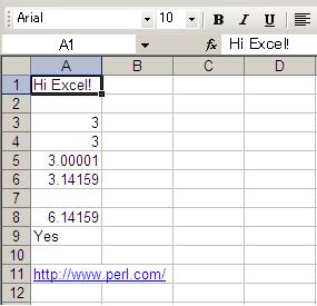
The following is a general example which demonstrates some features of working with multiple worksheets.
#!/usr/bin/ruby -w
require 'writeexcel'
# Create a new Excel workbook
workbook = WriteExcel.new('regions.xls')
# Add some worksheets
north = workbook.add_worksheet('North')
south = workbook.add_worksheet('South')
east = workbook.add_worksheet('East')
west = workbook.add_worksheet('West')
# Add a Format
format = workbook.add_format
format.set_bold
format.set_color('blue')
# Add a caption to each worksheet
workbook.sheets.each do |worksheet|
worksheet.write(0, 0, 'Sales', format)
end
# Write some data
north.write(0, 1, 200000)
south.write(0, 1, 100000)
east.write(0, 1, 150000)
west.write(0, 1, 100000)
# Set the active worksheet
south.activate
# Set the width of the first column
south.set_column(0, 0, 20)
# Set the active cell
south.set_selection(0, 1)
workbook.close
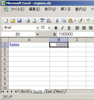
This example shows how to use a conditional numerical format with colours to indicate if a share price has gone up or down.
require 'writeexcel'
# Create a new workbook and add a worksheet
workbook = WriteExcel.new('stocks.xls')
worksheet = workbook.add_worksheet
# Set the column width for columns 1, 2, 3 and 4
worksheet.set_column(0, 3, 15)
# Create a format for the column headings
header = workbook.add_format
header.set_bold
header.set_size(12)
header.set_color('blue')
# Create a format for the stock price
f_price = workbook.add_format
f_price.set_align('left')
f_price.set_num_format('0.00')
# Create a format for the stock volume
f_volume = workbook.add_format
f_volume.set_align('left')
f_volume.set_num_format('#,##0')
# Create a format for the price change. This is an example of a
# conditional format. The number is formatted as a percentage. If it is
# positive it is formatted in green, if it is negative it is formatted
# in red and if it is zero it is formatted as the default font colour
# (in this case black). Note: the [Green] format produces an unappealing
# lime green. Try [Color 10] instead for a dark green.
#
f_change = workbook.add_format
f_change.set_align('left')
f_change.set_num_format('[Green]0.0%;[Red]-0.0%;0.0%')
# Write out the data
worksheet.write(0, 0, 'Company',header)
worksheet.write(0, 1, 'Price', header)
worksheet.write(0, 2, 'Volume', header)
worksheet.write(0, 3, 'Change', header)
worksheet.write(1, 0, 'Damage Inc.' )
worksheet.write(1, 1, 30.25, f_price ) # 30.25
worksheet.write(1, 2, 1234567, f_volume) # 1,234,567
worksheet.write(1, 3, 0.085, f_change) # 8.5% in green
worksheet.write(2, 0, 'Dump Corp.' )
worksheet.write(2, 1, 1.56, f_price ) # 1.56
worksheet.write(2, 2, 7564, f_volume) # 7,564
worksheet.write(2, 3, -0.015, f_change) # -1.5% in red
worksheet.write(3, 0, 'Rev Ltd.' )
worksheet.write(3, 1, 0.13, f_price ) # 0.13
worksheet.write(3, 2, 321, f_volume) # 321
worksheet.write(3, 3, 0, f_change) # 0 in the font color (black)
workbook.close
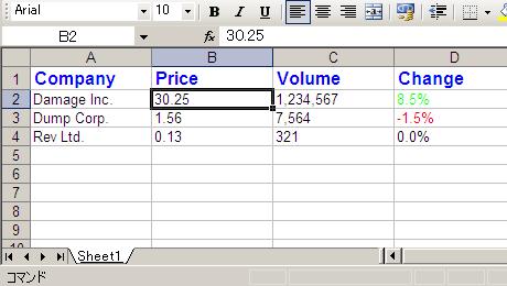
The following is a simple example of using functions.
#!/usr/bin/ruby -w
require 'writeexcel'
# Create a new workbook and add a worksheet
workbook = WriteExcel.new('stats.xls')
worksheet = workbook.add_worksheet('Test data')
# Set the column width for columns 1
worksheet.set_column(0, 0, 20)
# Create a format for the headings
format = workbook.add_format
format.set_bold
# Write the sample data
worksheet.write(0, 0, 'Sample', format)
worksheet.write(0, 1, 1)
worksheet.write(0, 2, 2)
worksheet.write(0, 3, 3)
worksheet.write(0, 4, 4)
worksheet.write(0, 5, 5)
worksheet.write(0, 6, 6)
worksheet.write(0, 7, 7)
worksheet.write(0, 8, 8)
worksheet.write(1, 0, 'Length', format)
worksheet.write(1, 1, 25.4)
worksheet.write(1, 2, 25.4)
worksheet.write(1, 3, 24.8)
worksheet.write(1, 4, 25.0)
worksheet.write(1, 5, 25.3)
worksheet.write(1, 6, 24.9)
worksheet.write(1, 7, 25.2)
worksheet.write(1, 8, 24.8)
# Write some statistical functions
worksheet.write(4, 0, 'Count', format)
worksheet.write(4, 1, '=COUNT(B1:I1)')
worksheet.write(5, 0, 'Sum', format)
worksheet.write(5, 1, '=SUM(B2:I2)')
worksheet.write(6, 0, 'Average', format)
worksheet.write(6, 1, '=AVERAGE(B2:I2)')
worksheet.write(7, 0, 'Min', format)
worksheet.write(7, 1, '=MIN(B2:I2)')
worksheet.write(8, 0, 'Max', format)
worksheet.write(8, 1, '=MAX(B2:I2)')
worksheet.write(9, 0, 'Standard Deviation', format)
worksheet.write(9, 1, '=STDEV(B2:I2)')
worksheet.write(10, 0, 'Kurtosis', format)
worksheet.write(10, 1, '=KURT(B2:I2)')
workbook.close
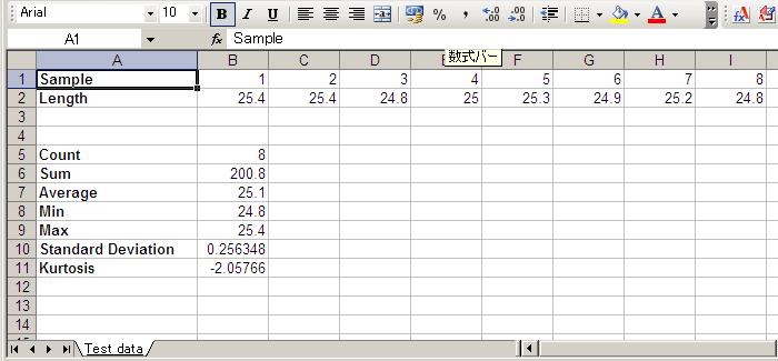
The following example converts a tab separated file called tab.txt into an Excel file called tab.xls.
#!/usr/bin/ruby -w
require 'rubygems'
require 'writeexcel'
File.open('tab.txt') do |f|
workbook = WriteExcel.new('tab.xls')
worksheet = workbook.add_worksheet
# Row and column are zero indexed
row = 0
f.read.each do |line|
col = 0
line.chomp.split("\t").each do |token|
worksheet.write(row, col, token)
col += 1
end
row += 1
end
workbook.close
end
Here is a complete example that demonstrates some of the available features when creating a chart.
#!/usr/bin/ruby -w
require 'rubygems'
require 'writeexcel'
workbook = WriteExcel.new( 'chart_area.xls' )
worksheet = workbook.add_worksheet
bold = workbook.add_format( :bold => 1 )
# Add the worksheet data that the charts will refer to.
headings = [ 'Number', 'Sample 1', 'Sample 2' ]
data = [
[ 2, 3, 4, 5, 6, 7 ],
[ 1, 4, 5, 2, 1, 5 ],
[ 3, 6, 7, 5, 4, 3 ]
]
worksheet.write( 'A1', headings, bold )
worksheet.write( 'A2', data )
# Create a new chart object. In this case an embedded chart.
chart = workbook.add_chart( :type => 'Chart::Area', :embedded => 1 )
# Configure the first series. (Sample 1)
chart.add_series(
:name => 'Sample 1',
:categories => '=Sheet1!$A$2:$A$7',
:values => '=Sheet1!$B$2:$B$7'
)
# Configure the second series. (Sample 2)
chart.add_series(
:name => 'Sample 2',
:categories => '=Sheet1!$A$2:$A$7',
:values => '=Sheet1!$C$2:$C$7'
)
# Add a chart title and some axis labels.
chart.set_title( :name => 'Results of sample analysis' )
chart.set_x_axis( :name => 'Test number' )
chart.set_y_axis( :name => 'Sample length (cm)' )
# Insert the chart into the worksheet (with an offset).
worksheet.insert_chart( 'D2', chart, 25, 10 )
workbook.close
This will produce a chart that looks like this:
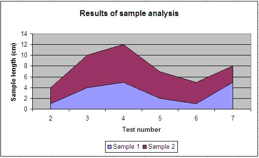
Here is a complete example that demonstrates some of the available features when creating a chart.
#!/usr/bin/ruby -w
require 'rubygems'
require 'writeexcel'
workbook = WriteExcel.new( 'chart_bar.xls' )
worksheet = workbook.add_worksheet
bold = workbook.add_format( :bold => 1 )
# Add the worksheet data that the charts will refer to.
headings = [ 'Number', 'Sample 1', 'Sample 2' ]
data = [
[ 2, 3, 4, 5, 6, 7 ],
[ 1, 4, 5, 2, 1, 5 ],
[ 3, 6, 7, 5, 4, 3 ],
]
worksheet.write( 'A1', headings, bold )
worksheet.write( 'A2', data )
# Create a new chart object. In this case an embedded chart.
chart = workbook.add_chart( :type => 'Chart::Bar', :embedded => 1 )
# Configure the first series. (Sample 1)
chart.add_series(
:name => 'Sample 1',
:categories => '=Sheet1!$A$2:$A$7',
:values => '=Sheet1!$B$2:$B$7'
)
# Configure the second series. (Sample 2)
chart.add_series(
:name => 'Sample 2',
:categories => '=Sheet1!$A$2:$A$7',
:values => '=Sheet1!$C$2:$C$7'
)
# Add a chart title and some axis labels.
chart.set_title( :name => 'Results of sample analysis' )
chart.set_x_axis( :name => 'Test number' )
chart.set_y_axis( :name => 'Sample length (cm)' )
# Insert the chart into the worksheet (with an offset).
worksheet.insert_chart( 'D2', chart, 25, 10 )
workbook.close
This will produce a chart that looks like this:
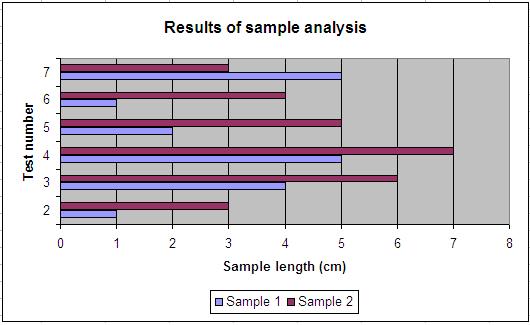
Here is a complete example that demonstrates some of the available features when creating a chart.
#!/usr/bin/ruby -w
require 'rubygems'
require 'writeexcel'
workbook = WriteExcel.new( 'chart_column.xls' )
worksheet = workbook.add_worksheet
bold = workbook.add_format( :bold => 1 )
# Add the worksheet data that the charts will refer to.
headings = [ 'Number', 'Sample 1', 'Sample 2' ]
data = [
[ 2, 3, 4, 5, 6, 7 ],
[ 1, 4, 5, 2, 1, 5 ],
[ 3, 6, 7, 5, 4, 3 ],
]
worksheet.write( 'A1', headings, bold )
worksheet.write( 'A2', data )
# Create a new chart object. In this case an embedded chart.
chart = workbook.add_chart( :type => 'Chart::Column', :embedded => 1 )
# Configure the first series. (Sample 1)
chart.add_series(
:name => 'Sample 1',
:categories => '=Sheet1!$A$2:$A$7',
:values => '=Sheet1!$B$2:$B$7'
)
# Configure the second series. (Sample 2)
chart.add_series(
:name => 'Sample 2',
:categories => '=Sheet1!$A$2:$A$7',
:values => '=Sheet1!$C$2:$C$7'
)
# Add a chart title and some axis labels.
chart.set_title( :name => 'Results of sample analysis' )
chart.set_x_axis( :name => 'Test number' )
chart.set_y_axis( :name => 'Sample length (cm)' )
# Insert the chart into the worksheet (with an offset).
worksheet.insert_chart( 'D2', chart, 25, 10 )
workbook.close
This will produce a chart that looks like this:
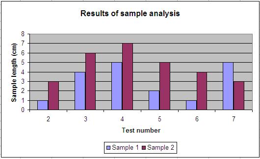
Here is a complete example that demonstrates some of the available features when creating a chart.
#!/usr/bin/ruby -w
require 'rubygems'
require 'writeexcel'
workbook = WriteExcel.new( 'chart_line.xls' )
worksheet = workbook.add_worksheet
bold = workbook.add_format( :bold => 1 )
# Add the worksheet data that the charts will refer to.
headings = [ 'Number', 'Sample 1', 'Sample 2' ]
data = [
[ 2, 3, 4, 5, 6, 7 ],
[ 1, 4, 5, 2, 1, 5 ],
[ 3, 6, 7, 5, 4, 3 ],
]
worksheet.write( 'A1', headings, bold )
worksheet.write( 'A2', data )
# Create a new chart object. In this case an embedded chart.
chart = workbook.add_chart( :type => 'Chart::Line', :embedded => 1 )
# Configure the first series. (Sample 1)
chart.add_series(
:name => 'Sample 1',
:categories => '=Sheet1!$A$2:$A$7',
:values => '=Sheet1!$B$2:$B$7'
)
# Configure the second series. (Sample 2)
chart.add_series(
:name => 'Sample 2',
:categories => '=Sheet1!$A$2:$A$7',
:values => '=Sheet1!$C$2:$C$7'
)
# Add a chart title and some axis labels.
chart.set_title( :name => 'Results of sample analysis' )
chart.set_x_axis( :name => 'Test number' )
chart.set_y_axis( :name => 'Sample length (cm)' )
# Insert the chart into the worksheet (with an offset).
worksheet.insert_chart( 'D2', chart, 25, 10 )
workbook.close
This will produce a chart that looks like this:
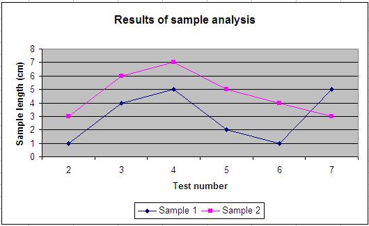
Here is a complete example that demonstrates some of the available features when creating a chart.
#!/usr/bin/ruby -w
require 'rubygems'
require 'writeexcel'
workbook = WriteExcel.new( 'chart_pie.xls' )
worksheet = workbook.add_worksheet
bold = workbook.add_format( :bold => 1 )
# Add the worksheet data that the charts will refer to.
headings = [ 'Category', 'Values' ]
data = [
[ 'Apple', 'Cherry', 'Pecan' ],
[ 60, 30, 10 ]
]
worksheet.write( 'A1', headings, bold )
worksheet.write( 'A2', data )
# Create a new chart object. In this case an embedded chart.
chart = workbook.add_chart( :type => 'Chart::Pie', :embedded => 1 )
# Configure the series.
chart.add_series(
:name => 'Pie sales data',
:categories => '=Sheet1!$A$2:$A$4',
:values => '=Sheet1!$B$2:$B$4'
)
# Add a title.
chart.set_title( :name => 'Popular Pie Types' )
# Insert the chart into the worksheet (with an offset).
worksheet.insert_chart( 'C2', chart, 25, 10 )
workbook.close
This will produce a chart that looks like this:
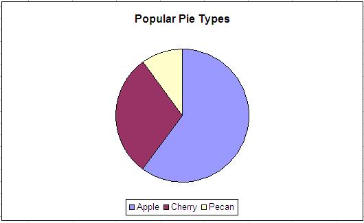
Here is a complete example that demonstrates some of the available features when creating a chart.
#!/usr/bin/ruby -w
require 'rubygems'
require 'writeexcel'
workbook = WriteExcel.new( 'chart_scatter.xls' )
worksheet = workbook.add_worksheet
bold = workbook.add_format( :bold => 1 )
# Add the worksheet data that the charts will refer to.
headings = [ 'Number', 'Sample 1', 'Sample 2' ]
data = [
[ 2, 3, 4, 5, 6, 7 ],
[ 1, 4, 5, 2, 1, 5 ],
[ 3, 6, 7, 5, 4, 3 ]
]
worksheet.write( 'A1', headings, bold )
worksheet.write( 'A2', data )
# Create a new chart object. In this case an embedded chart.
chart = workbook.add_chart( :type => 'Chart::Scatter', :embedded => 1 )
# Configure the first series. (Sample 1)
chart.add_series(
:name => 'Sample 1',
:categories => '=Sheet1!$A$2:$A$7',
:values => '=Sheet1!$B$2:$B$7'
)
# Configure the second series. (Sample 2)
chart.add_series(
:name => 'Sample 2',
:categories => '=Sheet1!$A$2:$A$7',
:values => '=Sheet1!$C$2:$C$7'
)
# Add a chart title and some axis labels.
chart.set_title( :name => 'Results of sample analysis' )
chart.set_x_axis( :name => 'Test number' )
chart.set_y_axis( :name => 'Sample length (cm)' )
# Insert the chart into the worksheet (with an offset).
worksheet.insert_chart( 'D2', chart, 25, 10 )
workbook.close
This will produce a chart that looks like this:
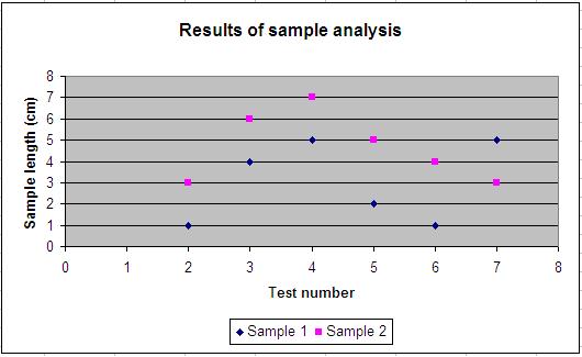
Here is a complete example that demonstrates some of the available features when creating a chart.
#!/usr/bin/ruby -w
require 'rubygems'
require 'writeexcel'
workbook = WriteExcel.new( 'chart_stock_ex.xls' )
worksheet = workbook.add_worksheet
bold = workbook.add_format( :bold => 1 )
date_format = workbook.add_format( :num_format => 'dd/mm/yyyy' )
# Add the worksheet data that the charts will refer to.
headings = [ 'Date', 'Open', 'High', 'Low', 'Close' ]
data = [
[ '2009-08-23', 110.75, 113.48, 109.05, 109.40 ],
[ '2009-08-24', 111.24, 111.60, 103.57, 104.87 ],
[ '2009-08-25', 104.96, 108.00, 103.88, 106.00 ],
[ '2009-08-26', 104.95, 107.95, 104.66, 107.91 ],
[ '2009-08-27', 108.10, 108.62, 105.69, 106.15 ]
]
worksheet.write( 'A1', headings, bold )
row = 1
data.each do |d|
worksheet.write( row, 0, d[0], date_format )
worksheet.write( row, 1, d[1] )
worksheet.write( row, 2, d[2] )
worksheet.write( row, 3, d[3] )
worksheet.write( row, 4, d[4] )
row += 1
end
# Create a new chart object. In this case an embedded chart.
chart = workbook.add_chart( :type => 'Chart::Stock', :embedded => 1 )
# Add a series for each of the Open-High-Low-Close columns.
chart.add_series(
:categories => '=Sheet1!$A$2:$A$6',
:values => '=Sheet1!$B$2:$B$6',
:name => 'Open'
)
chart.add_series(
:categories => '=Sheet1!$A$2:$A$6',
:values => '=Sheet1!$C$2:$C$6',
:name => 'High'
)
chart.add_series(
:categories => '=Sheet1!$A$2:$A$6',
:values => '=Sheet1!$D$2:$D$6',
:name => 'Low'
)
chart.add_series(
:categories => '=Sheet1!$A$2:$A$6',
:values => '=Sheet1!$E$2:$E$6',
:name => 'Close'
)
# Add a chart title and some axis labels.
chart.set_title( :name => 'Open-High-Low-Close' )
chart.set_x_axis( :name => 'Date' )
chart.set_y_axis( :name => 'Share price' )
# Insert the chart into the worksheet (with an offset).
worksheet.insert_chart( 'F2', chart, 25, 10 )
workbook.close
This will produce a chart that looks like this:
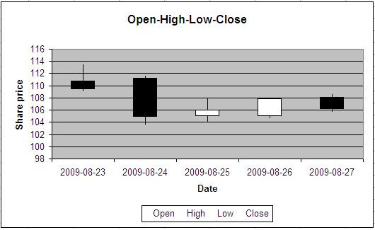
The following is a description of the example files that are provided in the standard WriteExcel distribution. They demonstrate the different features and options of the module.
Getting started
===============
a_simple.rb A get started example with some basic features.
demo.rb A demo of some of the available features.
regions.rb A simple example of multiple worksheets.
stats.rb Basic formulas and functions.
formats.rb All the available formatting on several worksheets.
bug_report.rb A template for submitting bug reports.
Advanced
========
autofilter.rb Examples of worksheet autofilters.
bigfile.rb Write past the 7MB limit with OLE::Storage_Lite.
chart_area.rb A demo of area style charts.
chart_bar.rb A demo of bar (vertical histogram) style charts.
chart_column.rb A demo of column (histogram) style charts.
chart_legend.rb A demo of chart with/without legend.
chart_line.rb A demo of line style charts.
chart_pie.rb A demo of pie style charts.
chart_scatter.rb A demo of scatter style charts.
chart_stock.rb A demo of stock style charts.
chess.rb An example of reusing formatting via properties.
colors.rb A demo of the colour palette and named colours.
comments1.rb Add comments to worksheet cells.
comments2.rb Add comments with advanced options.
copyformat.rb Example of copying a cell format.
data_validate.rb An example of data validation and dropdown lists.
date_time.rb Write dates and times with write_date_time.
defined_name.rb Example of how to create defined names.
formula_result.rb Formulas with user specified results.
header.rb Examples of worksheet headers and footers.
hide_sheet.rb Simple example of hiding a worksheet.
hyperlink.rb Shows how to create web hyperlinks.
images.rb Adding images to worksheets.
indent.rb An example of cell indentation.
merge1.rb A simple example of cell merging.
merge2.rb A simple example of cell merging with formatting.
merge3.rb Add hyperlinks to merged cells.
merge4.rb An advanced example of merging with formatting.
merge5.rb An advanced example of merging with formatting.
merge6.rb An example of merging with Unicode strings.
outline.rb An example of outlines and grouping.
outline_collapsed.rb An example of collapsed outlines.
panes.rb An examples of how to create panes.
password_protection.rb An example of sheet protection by password.
properties.rb Add document properties to a workbook.
properties_jp.rb Add document properties in Japanese to a workbook.
protection.rb Example of cell locking and formula hiding.
repeat.rb Example of writing repeated formulas.
right_to_left.rb Change default sheet direction to right to left.
row_wrap.rb How to wrap data from one worksheet onto another.
sales.rb An example of a simple sales spreadsheet.
stats.rb A simple example of how to use functions.
stocks.rb Demonstrates conditional formatting.
tab_colors.rb Example of how to set worksheet tab colours.
write_arrays.rb Example of writing 1D or 2D arrays of data.
The following limits are imposed by Excel:
Description Limit
----------------------------------- ------
Maximum number of chars in a string 32767
Maximum number of columns 256
Maximum number of rows 65536
Maximum chars in a sheet name 31
Maximum chars in a header/footer 254
WriteExcel will work on the majority of Windows, UNIX and Macintosh platforms.
p [1.2345].pack('d').unpack('C*').map {|c| sprintf("%#02x", c)}.join(' ')
should give (or in reverse order):
0x8d 0x97 0x6e 0x12 0x83 0xc0 0xf3 0x3f
In general, if you don't know whether your system supports a 64 bit IEEE float or not, it probably does.
The following is some general information about the Excel binary format for anyone who may be interested.
Excel data is stored in the "Binary Interchange File Format" (BIFF) file format. Details of this format are given in "Excel 97-2007 Binary File Format Specification" http://www.microsoft.com/interop/docs/OfficeBinaryFormats.mspx.
Daniel Rentz of OpenOffice.org has also written a detailed description of the Excel workbook records, see http://sc.openoffice.org/excelfileformat.pdf.
Charles Wybble has collected together additional information about the Excel file format. See "The Chicago Project" at http://chicago.sourceforge.net/devel/.
The BIFF data is stored along with other data in an OLE Compound File. This is a structured storage which acts like a file system within a file. A Compound File is comprised of storages and streams which, to follow the file system analogy, are like directories and files.
The OLE format is explained in the "Windows Compound Binary File Format Specification" http://www.microsoft.com/interop/docs/supportingtechnologies.mspx
The Digital Imaging Group have also detailed the OLE format in the JPEG2000 specification: see Appendix A of http://www.i3a.org/pdf/wg1n1017.pdf.
Please note that the provision of this information does not constitute an invitation to start hacking at the BIFF or OLE file formats. There are more interesting ways to waste your time. ;-)
MIT Lisence.
Original perl module : Copyright MM-MMX, John McNamara. All Rights Reserved. This module is free software. It may be used, redistributed and/or modified under the same terms as Perl itself.
writeexcel Rubygem : Copyright(c) Hideo NAKAMURA. All Rights Reserved. This module is free software. It may be used, redistributed and/or modified under the same terms as Ruby itself.